Log Distance Path Loss or Log Normal Shadowing Model

Log distance path loss model

Log distance path loss model is an extension to the Friis free space model. It is used to predict the propagation loss for a wide range of environments, whereas, the Friis free space model is restricted to unobstructed clear path between the transmitter and the receiver. The model encompasses random shadowing effects due to signal blockage by hills, trees, buildings etc. It is also referred as log normal shadowing model.

In the far field region of the transmitter, for distances beyond $latex d_f$, if $latex P_L(d_0)$ is the path loss at a distance $latex d_0$ meters from the transmitter, then the path loss at an arbitrary distance $latex d>d_0$ is given by

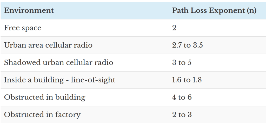
where, $latex P_L(d)$ is the path loss at an arbitrary distance $latex d$ meters, $latex n$ is the path loss exponent that depends on the type of environment, as given in Table below. Also, $latex \chi$ is a zero-mean Gaussian distributed random variable with standard deviation $latex \sigma$ expressed in $latex dB$, used only when there is a shadowing effect. The reference path loss $latex P_L(d_0)$, also called close-in reference distance, is obtained by using Friis path loss equation (equation 2 in this post) or by field measurements at $latex d_0$. Typically, $latex d_0=1m$ to $latex 10m$ for microcell and $latex d_0 = 1\;Km$ for a large cell.

[table id=36 /]

The path-loss exponent (PLE) values given in Table below are for reference only. They may or may not fit the actual environment we are trying to model. Usually, PLE is considered to be known a-priori, but mostly that is not the case. Care must be taken to estimate the PLE for the given environment before design and modeling. PLE is estimated by equating the observed (empirical) values over several time instants, to the established theoretical values. Refer [1] for a literature on PLE estimation in large wireless networks.

logNormalShadowing.m: Function to model Log-normal shadowing (Refer the book for the Matlab code – click here)

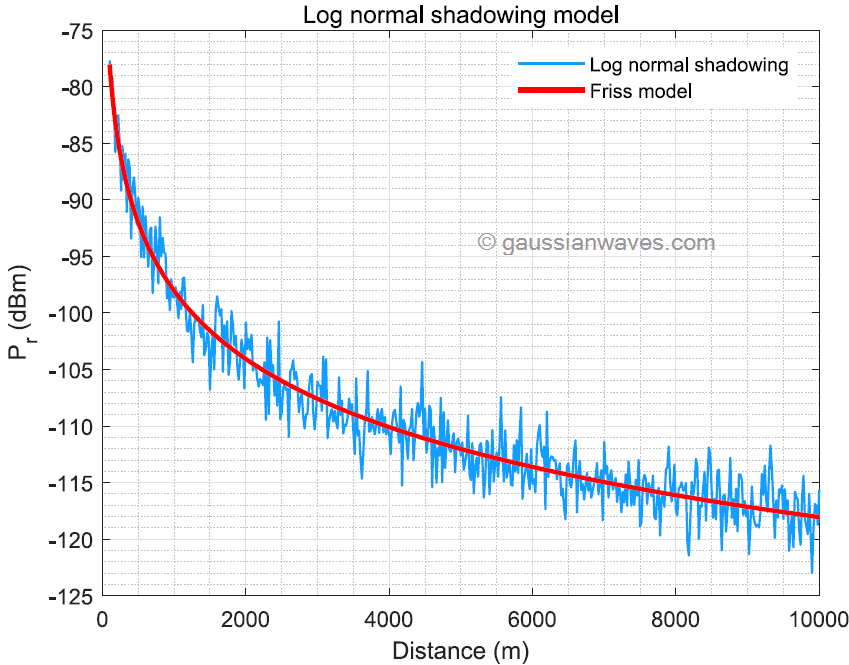
The function to implement log-normal shadowing is given above and the test code is given next. Figure 1 shows the received signal when there is no shadowing effect and the case where shadowing exists. The r

The function to implement log-normal shadowing is given above and the test code is given next. Figure 1 above shows the received signal power when there is no shadowing effect and the case when shadowing exists. The results are generated for an environment with PLE n = 2, frequency of transmission f = 2.4 GHz, reference distance d₀ = 1 m and standard deviation of the log-normal shadowing σ = 2dB. Results clearly show that the log-normal shadowing introduces randomness in the received signal power, which may put us close to reality.

log_distance_model_test.m: Simulate Log Normal Shadowing for a range of distances

Pt_dBm=0; %Input transmitted power in dBm
Gt_dBi=1; %Gain of the Transmitted antenna in dBi
Gr_dBi=1; %Gain of the Receiver antenna in dBi
f=2.4e9; %Transmitted signal frequency in Hertz
d0=1; %assume reference distance = 1m
d=100*(1:0.2:100); %Array of distances to simulate
L=1; %Other System Losses, No Loss case L=1
sigma=2;%Standard deviation of log Normal distribution (in dB)
n=2; % path loss exponent
%Log normal shadowing (with shadowing effect)
[PL_shadow,Pr_shadow] = logNormalShadowing(Pt_dBm,Gt_dBi,Gr_dBi,f,d0,d,L,sigma,n);
figure;plot(d,Pr_shadow,'b');hold on;
%Friis transmission (no shadowing effect)
[Pr_Friss,PL_Friss] = FriisModel(Pt_dBm,Gt_dBi,Gr_dBi,f,d,L,n);
plot(d,Pr_Friss,'r');grid on;
xlabel('Distance (m)'); ylabel('P_r (dBm)');
title('Log Normal Shadowing Model');legend('Log normal shadowing','Friss model');

Rate this article: [ratings]

References

[1] Srinivasan, S.; Haenggi, M., Path loss exponent estimation in large wireless networks, Information Theory and Applications Workshop, pp. 124 – 129, Feb 2009.↗

Topic in this chapter

• Introduction to Large scale propagation models
• Friis free space propagation model
• Log distance path loss model
• Two ray ground reflection model
• Modeling diffraction loss
  • Single knife-edge diffraction model
  • Fresnel zones
• Hata Okumura model for outdoor propagation

Books by the author

[table id=23 /]