Introduction to Multiple Antenna Systems

Introduction

If you have ever watched a phone cling to a call while you walk behind a building, you have already met fading. The wave that left the base station did not travel on one tidy path; it bounced and diffracted, and the copies interfere so the received amplitude wanders with time and position. With a single antenna you have only one look at that random process. When the fade is deep, there is nowhere to hide.

Multiple-antenna systems—MIMO when both ends use several radiators—give you a second look at the same information, or several spatial pipes for new information. This opening note sets vocabulary and motivation. We will not yet optimise combiners or compute capacity integrals. The question for now is simpler: what problem are multiple antennas trying to solve, and how do we write the channel so that later calculations make sense?

Motive: reliability, rate, or both?

Standards ask for two things that pull against each other. Reliability wants copies of the same bit to survive deep fades. Rate wants fresh bits in the same time–frequency resource. Spatial degrees of freedom can be spent either way:

• Spatial diversity spends antennas on reliability: send or receive redundant versions of one symbol so that not all versions fade together.
• Spatial multiplexing spends antennas on rate: send independent streams that the receiver untangles using the structure of the channel matrix.

Beamforming and phased arrays, which we treat in a separate series, are a third use of the same geometry: point energy where you want it. Keep the distinction clear. Diversity and multiplexing are communication uses of space; beamforming is an array-processing use. Real systems mix all three.

Technical development: from SISO to a matrix channel

The SISO baseline

Start with one transmit and one receive antenna. After matched filtering and sampling at the symbol rate in flat fading, the observation collapses to a scalar

\[y = h x + n,\]

where \(x\) is the complex baseband symbol, \(n\) is circularly symmetric Gaussian noise, and \(h\) is the complex channel gain for that coherence block. If the receiver knows \(h\), the Shannon rate for that realisation is \(\log_2(1+|h|^2 P/N_0)\). The trouble is that \(|h|\) is random. On a Rayleigh model, \(|h|^2\) is exponential, and with non-negligible probability it sits near zero.

Several antennas, one matrix

Now place \(N_t\) antennas at the transmitter and \(N_r\) at the receiver. In the same flat-fading, symbol-sampled setting the natural description is a matrix equation

\[\mathbf{y} = \mathbf{H}\mathbf{x} + \mathbf{n}, \qquad \mathbf{H}\in\mathbb{C}^{N_r\times N_t}.\]

The entry \(H_{ij}\) is the gain from transmit antenna \(j\) to receive antenna \(i\). Under rich scattering with well-separated antennas one often models the entries as i.i.d. \(\mathcal{CN}(0,1)\). That is an idealisation, but it is the right idealisation to learn on: it maximises the typical rank of \(\mathbf{H}\) and therefore the potential for multiplexing.

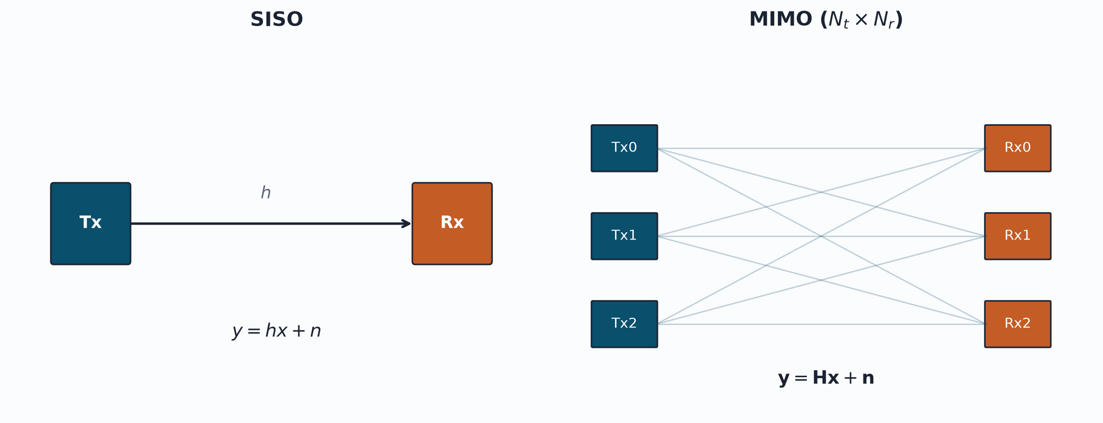
Figure 1 says something simple: every receive antenna hears a linear mixture of every transmit antenna. Depending on the mode, the receiver either combines those mixtures for reliability or untangles them for rate.

How this achieves the motive

Diversity works because deep fades on independent paths rarely coincide. If two receive antennas see uncorrelated \(h_1\) and \(h_2\), the chance that both are simultaneously weak is the product of the individual probabilities—hence the outage curves that fall as a power of SNR later in this path.

Multiplexing works when \(\mathbf{H}\) has several significant singular values. The SVD \(\mathbf{H}=\mathbf{U}\boldsymbol{\Sigma}\mathbf{V}^H\) exposes parallel gains; waterfilling or equal power on those modes turns space into rate. If the singular values collapse (keyhole channels, strong correlation), multiplexing evaporates and you are better off spending the antennas on diversity or beamforming.

Sample simulation: draw a channel and look at it

Before capacity formulas, it helps to inspect one channel draw. The listing below forms a \(4\times 4\) i.i.d. Rayleigh matrix and prints its singular values. Run it several times and note how the spread of \(\sigma_i\) changes from draw to draw.

import numpy as np

Nt, Nr = 4, 4
rng = np.random.default_rng(0)
H = (rng.standard_normal((Nr, Nt)) + 1j * rng.standard_normal((Nr, Nt))) / np.sqrt(2)
s = np.linalg.svd(H, compute_uv=False)
print("singular values:", np.round(s, 3))
print("condition number:", round(s.max() / s.min(), 2))
print("Frobenius energy:", round(np.linalg.norm(H, "fro") ** 2, 3), " (expect ~ Nt*Nr = 16)")

Sample results

For seed 0 you should see a decaying staircase of singular values and a Frobenius energy near \(16\). A large condition number means the weakest mode is fragile: at modest SNR you effectively have fewer than four streams. That is why capacity articles average over many draws of \(\mathbf{H}\) rather than relying on a single matrix.

Next topic

The next article takes up the design choice directly: when should spatial degrees of freedom go to diversity versus spatial multiplexing? After that we treat receive-only arrays (SIMO), then selection combining and MRC, and in a parallel path we develop capacity from SISO fading up to MIMO.

References

1. D. Tse and P. Viswanath, Fundamentals of Wireless Communication, Cambridge University Press, Cambridge, UK, 2005.
2. A. Goldsmith, Wireless Communications, Cambridge University Press, Cambridge, UK, 2005.
3. A. Paulraj, R. Nabar, and D. Gore, Introduction to Space-Time Wireless Communications, Cambridge University Press, Cambridge, UK, 2003.

Frequently asked questions

What problem do multiple antennas solve that a single antenna cannot? A single-antenna link has only one observation of a fading channel. When that fade is deep, the link has no alternative path. Multiple antennas supply either redundant observations of the same symbol (spatial diversity) or additional spatial degrees of freedom for independent streams (spatial multiplexing), and in practice a mixture of both.

How is the MIMO channel written mathematically? After matched filtering in flat fading, the baseband model is the matrix equation \(\mathbf{y}=\mathbf{Hx}+\mathbf{n}\), where \(H_{ij}\) is the complex gain from transmit antenna \(j\) to receive antenna \(i\). Under rich scattering the entries are often modelled as i.i.d. circularly symmetric complex Gaussian random variables.

What do the singular values of \(\mathbf{H}\) tell you? The singular values are the gains of the parallel spatial modes exposed by the SVD. A large condition number means some modes are weak: at modest SNR you effectively have fewer streams than antennas. That is why capacity analyses average over many channel draws rather than trusting one realisation.

How do diversity, multiplexing, and beamforming differ? Diversity spends antennas on reliability; multiplexing spends them on rate; beamforming (or phased-array processing) points energy in preferred directions. Wireless standards combine all three through rank adaptation, codebook precoding, and space-time or space-frequency coding.