Two flavors of MIMO implementation – spatial multiplexing and spatial diversity – were discussed in the previous article. In that, it was mentioned that the reliability of a MIMO system is governed by diversity and the capacity of the link is governed by degrees of freedom.
Channel State Information (CSI)
Multiple data streams can be spatially multiplexed over the M transmit antennas and are received by the N receiver antennas. Spatially multiplexing increases the capacity of the link, since multiple data streams are transmitted over the same available frequency band. On the other hand, antenna diversity systems (dubbed as MIMO using diversity) merely improve the reliability of the link.
But the question of whether the transmission of multiple streams of data over multiple antenna really works, depends on the actual geometry of the antenna systems. Transmission of independent data streams over multiple antennas depends on the correlation factor that measures the influence of the spatially separated signals over each other. One way to eliminate correlation (there by mutual influence of spatially separated signals) is to use orthogonally polarized antennas (one antenna is horizontally polarized and the other is vertically polarized) that sufficiently separate the signals in spatial dimension.
Finally, the transmission matrix (also called Channel State Information (CSI) ) determines the suitability of MIMO techniques and influences the capacity to a great extent. In a SISO channel, the channel state information is constant and does not change from bit to bit. Thus the knowledge of CSI in a SISO link is often not needed as it is characterized by steady state SNR. In the case of rapid fading channels, the channel state information varies rapidly and we may think of employing MIMO to break the channel variations into spatially separated sub channels. Thus, the knowledge channel state information (at transmitter or receiver) will open up the possibility of incorporating this information in intelligent system design.
In a MIMO configuration, a typical CSI matrix is formed by transmitting a symbol (say value ‘1’) from each of the transmitting antenna and its response on the multiple receiving antennas are noted. For example, in a  configuration, at some time instant, we transmit the voltage ‘1’ from the first antenna and record its response on the three receiving antennas. Lets say the three receiver antennas picks up the following voltage values – [0.8, 0.7, 0.9 ].
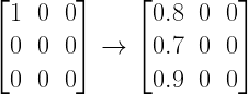
At the same time instant, the procedure is repeated for other transmit antennas and the response of multiple receive antennas are recorded. A complete CSI matrix is shown below

In this method, the transmitter transmits the data blindly and the receiver constructs the CSI matrix. This method of transmission is called open loop transmission scheme and are not generally effective. From the sample CSI matrix above, it can be noted that the transmission through antenna 2 is not effective (note the low voltage values recorded at the receiver antennas (second column on the right) ) the receiver may feed back the CSI matrix to the transmitter and the transmitter may decide not to transmit on antenna 2, there by saving power. This is an example for closed loop diversity scheme. In this way the knowledge of CSI opens up the possibility for intelligent communication.
The CSI matrix shown above contain only real numbers that describe the amplitude variations. In reality the CSI matrix contains elements that are complex and they describe both the amplitude and phase variations of the link.

MIMO channel Model
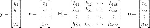
A channel model is needed to properly assess a MIMO channel. In MIMO, the system configuration typically contains M antennas at the transmitter and N antennas at the receiver front end as illustrated in the following figure.

Here, each receiver antenna receives not only the direct signal intended for it, but also receives a fraction of signal from other propagation paths. Thus, the channel response is expressed as a transmission matrix H. The direct path formed between antenna 1 at the transmitter and the antenna 1 at the receiver is represented by the channel response  . The channel response of te path formed between antenna 1 in the transmitter and antenna 2 in the receiver is expressed as
  and so on. Thus, the channel matrix is of dimension
  .
.
The received vector  is expressed in terms of the channel transmission matrix
  , the input vector
  and noise vector
  as
as

where the various symbols are
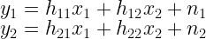
Note that the response of the MIMO link is expressed as a set of linear equations. For a simple  MIMO configuration, the received signal vector is expressed as

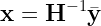
The receiver has to solve this set of equations to find out what was transmitted ( ). The stability of the solution depends on the condition number of the transmission matrix (CSI).
Condition Number
Solving a set of linear equation has its own challenges – rounding effects and how bad a matrix is. Obviously an on-board computer will be solving those equations. Storage of co-efficients in computer memory is prone to fixed point effects or rounding. Pivoting is method that address the problems with rounding effects when Gauss Jordan elimination procedure is used. It makes sure that the Gaussian elimination procedure proceeds as intended. Problems do occur even without rounding effects. A small change in input can cause drastic difference in the solution. In the set of linear equations mentioned above, the variations to the solutions can be effected by the noise term. The solution should be robust against variations in the noise (at-least to certain extent). The sensitivity of the solution to small changes in the input data is measured by condition number of the transmission matrix ( ). It indicates the stability of the solution ( ) to small change in incoming data ( ).
At the receiver, the received data is known and is often corrupted by noise. Let’s consider the received vector  that is corrupted by noise . Thus the system of linear equations is given as
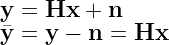
Also, the channel transmission matrix is usually estimated approximately. The solution is obtained as
The solution to the above equation may or may not exist and may or may not be unique. Let’s consider a symmetric transmission matrix  . From matrix and linear algebra[1][2], if the input is arbitrary (as is the case here), an unique solution is possible only if the matrix is non-singular. The condition number (
 ) of a non-singular matrix is given as
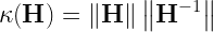
where  denotes the matrix norm[1]. The condition number measures the relative sensitivity of the solutions to the changes in the input data ( ). The changes to the solution can be expressed as
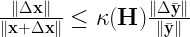
where  represents the change in the solution,
  represent a change in the observed or received samples and
  denotes the condition number of the transmission matrix.
In other words, a small change in the input data gets multiplied by the condition number and produces changes in the output (solution). Thus high condition number is bad and is regarded as ill-conditioned matrix. An ill-conditioned matrix will behave similar to a singular matrix which will not render any solution or will give infinite non-unique solutions (see the table below).
Translating to the problem of transmission by MIMO, the ability to transmit multiple data streams across a MIMO channel – relies on the ability of the receiver to solve the system of linear equations in an unambiguous and stable way. Thus the condition number of the transmission matrix affects the suitability of spatial multiplexing in a MIMO link. A well-conditioned matrix (low condition number) allows reliable transmission of spatially multiplexed signal, whereas an ill-conditioned matrix makes it difficult to do so.
Additionally, the rank of the transmission matrix –  indicates how many data streams can be spatially multiplexed on a MIMO link. Thus the rank and the condition number of the transmission matrix play an important role in a MIMO system design.
Some useful prepositions
Existence and uniqueness
Given a system of linear equations  , existence and uniqueness of the solution depends on whether the matrix is singular or non-singular. It also depends on the input vector for the singular case.

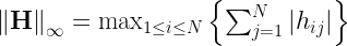
Matrix norm[1]
Matrix norm (the maximum absolute row sum) is calculated as
Non-Singular Matrix
An matrix is non-singular if it has any of the following properties
● Inverse  exists
● 
● 
● For any vector  ,
,
Rate this article : 
 (32 votes, average: 4.25 out of 5)
References
[1] Stephen Boyd, Symmetric matrices, quadratic forms, matrixnorm, and SVD, Stanford university, EE263 Autumn 2007-08.↗
[2] Review of Linear Algebra.↗
Books by the author
 Wireless Communication Systems in Matlab Second Edition(PDF)  (172 votes, average: 3.66 out of 5) (172 votes, average: 3.66 out of 5) |  Digital Modulations using Python (PDF ebook) (127 votes, average: 3.58 out of 5) |  Digital Modulations using Matlab (PDF ebook) (134 votes, average: 3.63 out of 5) |
| Hand-picked Best books on Communication Engineering Best books on Signal Processing |
||
How can this article be cited? Does this text appear in one of your books?
This article is not part of any of my books. It is only available here.
To cite, please use the following format:
Viswanathan Mathuranathan, “Characterizing a MIMO channel – Channel State Information (CSI) and Condition number”, Gaussianwaves.com, August 20, 2014, https://www.gaussianwaves.com/2014/08/characterizing-a-mimo-channel/
Thank you