Let’s see how to design a simple digital FIR filter to reject unwanted frequencies in an incoming signal. As a per-requisite, I urge you to read through this post: Introduction to digital filter design
Background on transfer function
The transfer function of a system provides the underlying support for ascertaining vital system response characteristics without solving the difference equations of the system. As mentioned earlier, the transfer function of a generic filter in Z-domain is given by ratio of polynomials in z
\[H(z) = \frac{ \displaystyle{\sum_{i=0}^{M} b_k z^{-1}}}{ 1 + \displaystyle{\sum_{i=1}^{N} a_k z^{-1}} } \quad\quad (1)\]The values of z when H(z) =0 are called zeros of H(z). The values of z when H(z) = ∞ are called poles of H(z).
It is often easy to solve for zeros {zi} and poles {pj}, when the polynomials in the numerator and denominator are expressed as resolvable factors.
\[H(z) = \frac{ \displaystyle{\sum_{i=0}^{M} b_k z^{-1}}}{ 1 + \displaystyle{\sum_{i=1}^{N} a_k z^{-1}} } = \frac{N(z)}{D(z)} = \frac{b_M}{a_N} \frac{(z – z_1)(z – z_2)\cdots (z – z_M)}{(z – p_1)(z – p_2)\cdots (z – p_N)} \quad\quad (2) \]The zeros {zi} are obtained by finding the roots of the equation
\[N(z) = 0 \quad\quad (3)\]The poles {pj} are obtained by finding the roots of the equation
\[D(z) = 0 \quad\quad (4) \]Pole-zero plots are suited for visualizing the relationship between the Z-domain and the frequency response characteristics. As mentioned before, the frequency response of the system H(e jω) can be computed by evaluating the transfer function H(z) at specific values of z = e jω. Because the frequency response is periodic with period 2π, it is sufficient to evaluate the frequency response for the range -π <= ω < π (that is one loop around the unit circle on the z-plane starting from z=-1 and ending at the same point).
FIR filter design
FIR filters contain only zeros and no poles in the pole-zero plot (in fact all the poles sit at the origin for a causal FIR). For an FIR filter, the location of zeros of H(z) on the unit-circle nullifies specific frequencies. So, to design an FIR filter to nullify specific frequency ω, we just have to place the zeros at corresponding locations on the unit circle (z=ejω) where the gain of the filter needs to be 0. Let’s illustrate this using an example.
For this illustration, we would use this audio file as an input to the filtering system. As a first step in the filter design process, we should understand the nature of the input signal. Discrete-time Fourier transform (DTFT) is a tool for analyzing the frequency domain characteristics of the given signal.
The following function is used to compute the DTFT of the sequence read from the audio file.
import numpy as np
import matplotlib.pyplot as plt

from math import ceil,log,pi,cos
from scipy.fftpack import fft,fftfreq,fftshift

def compute_DTFT(x,M=0):
    """
    Compute DTFT of the given sequence x
    M is the desired length for computing DTFT (optional).
    Returns the DTFT X[k] and corresponding frequencies w (omega) arranged as -pi to pi
    """
    N = max(M,len(x))
    N = 2**(ceil(log(N)/log(2)))

    X = fftshift(fft(x,N))
    w = 2*pi*fftshift(fftfreq(N))
    return (X,w)
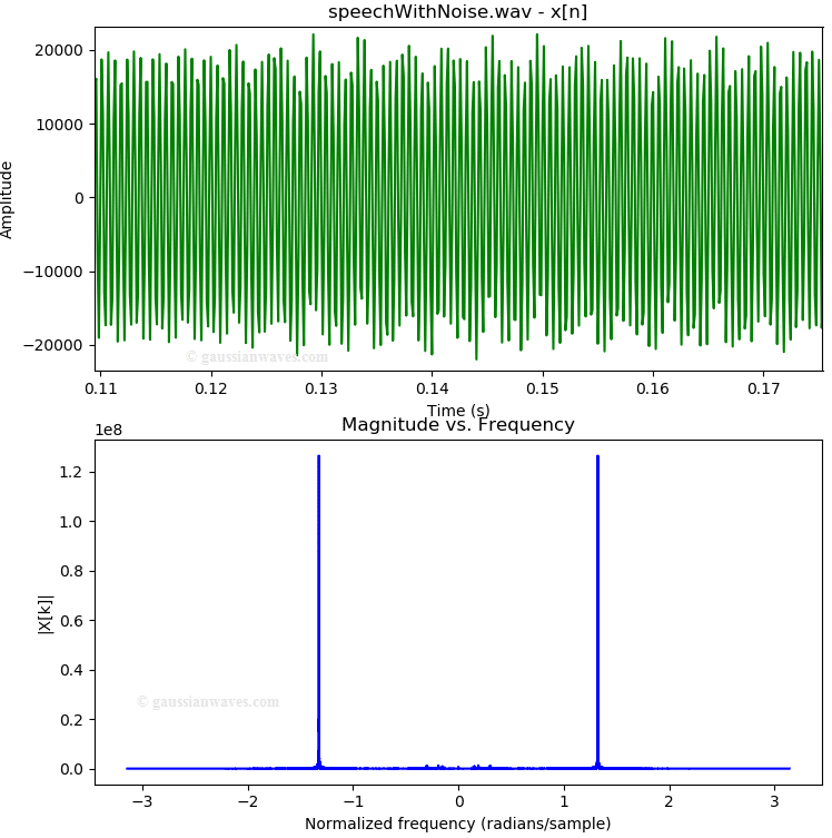
Let’s read the audio file, load the samples as a signal sequence $latex x$, and plot the sequence in time-domain/frequency domain (using DTFT).
from scipy.io.wavfile import read

samplerate, x = read('speechWithNoise.wav')
duration = len(x)/samplerate
time = np.arange(0,duration,1/samplerate)

fig1, (ax1,ax2) = plt.subplots(nrows=2,ncols=1)
ax1.plot(time,x)
ax1.set_xlabel('Time (s)')
ax1.set_ylabel('Amplitude')
ax1.set_title('speechWithNoise.wav - x[n]')

(X,w)= compute_DTFT(x)
ax2.plot(w,abs(X))
ax2.set_xlabel('Normalized frequency (radians/sample)')
ax2.set_ylabel('|X[k]|')
ax2.set_title('Magnitude vs. Frequency')The magnitude vs. frequency plot simply shows huge spikes at θ=±1.32344 radians. The location of the spikes are captured by using the numpy.argmax↗ function.
maxIndex = np.argmax(X)
theta = w[maxIndex]
print(theta)
Since a sinusoid can be mathematically represented as
\[x[n] = cos (\theta n) = \frac{1}{2}\left( e^{j \theta n} + e^{-j \theta n }\right) \quad\quad (5)\]The two spikes at θ=±1.32344 radians in the frequency domain, will manifest as a sinusoidal signal in the time domain.
Zooming in the area between θ= ±0.4 radians, the frequency domain plot reveals a hidden signal.
Now, our goal is to design an FIR filter that should reject the sinusoid at θ=±1.32344 radians, so that only the hidden signal gets filtered in.
Since the sinusoid that we want to reject is occurring at some θ radians in the frequency domain, for the FIR filter design, we place two zeros at
\[z_1 = e^{j \theta} \quad\quad z_2 = e^{-j \theta}\quad\quad (6)\]Therefore, the transfer function of the filter system is given by
\[\begin{aligned} H_f(z) &= \left( 1 – z_1 z^{-1}\right)\left(1 – z_2 z^{-1} \right) \\ &= \left( 1 – e^{j \theta} z^{-1}\right)\left(1 -e^{-j \theta}z^{-1} \right) \\ & = 1 – 2\;cos\left(\theta\right)z^{-1} + z^{-2} \end{aligned}\]This is a second order FIR filter. The coefficients of the filter are
\[b_0 = 1,\; b_1 = – 2 cos (\theta),\; b_2 = 1 \text{ and } a_0=1\]For the given problem, to should reject the sinusoid at θ=±1.32344 radians, we set θ=1.32344 in the filter coefficients above.
Filter in action
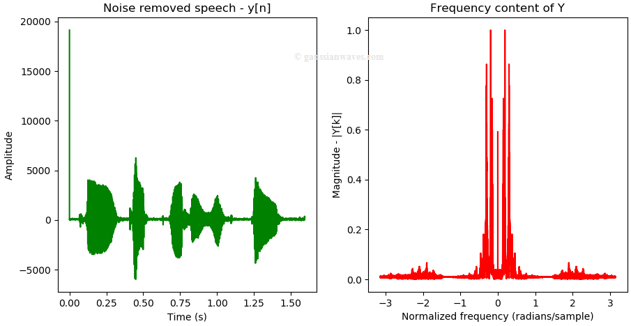
Filter the input audio signal through the designed filter and plot the filtered output in time-domain and frequency domain. The lfilter function from scipy.signal package↗ is utilized for the filtering operation.
from scipy.signal import lfilter
y_signal = lfilter(b, a, x)
fig3, (ax3,ax4) = plt.subplots(nrows=1,ncols=2)
ax3.plot(time,y_signal,'g')
ax3.set(title='Noise removed speech - y[n]',xlabel='Time (s)',ylabel='Amplitude')

(Y,w)= compute_DTFT(y_signal)
ax4.plot(w,abs(Y)/max(abs(Y)),'r')
ax4.set(title='Frequency content of Y',xlabel='Normalized frequency (radians/sample)',ylabel='Magnitude - |Y[k]|')
The filter has effectively removed the sinusoidal noise, as evident from both time-domain and frequency domain plots.
Save the filtered output signal as .wav file for audio playback
from scipy.io.wavfile import write
output_data = np.asarray(y_signal, dtype=np.int16)#convert y to int16 format
write("noise_removed_output.wav", samplerate, output_data)
Characteristics of the designed filter
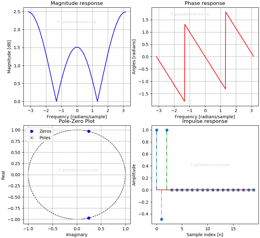
Let’s compute the double sided frequency response of the designed FIR filter. The frequency response of the designed FIR digital filter is computed using freqz function from the scipy.signal package↗.
from scipy.signal import freqz
b = [1,-2*cos(theta),1] #filter coefficients
a = [1]
w, h = freqz(b,a,whole=True)#frequency response h[e^(jw)]
#whole = True returns output for whole range 0 to 2*pi
#To plot double sided response, use fftshift
w = w - 2*np.pi*(w>=np.pi) #convert to range -pi to pi
w = fftshift(w)
h = fftshift(h)
Plot the magnitude response, phase response, pole-zero plot and the impulse response of the designed filter.
#Plot Magnitude-frequency response
fig2, (ax) = plt.subplots(nrows=2,ncols=2)
ax[0,0].plot(w,abs(h),'b')
ax[0,0].set(title='Magnitude response',xlabel='Frequency [radians/sample]',ylabel='Magnitude [dB]')
ax[0,0].grid();ax[0,0].axis('tight');

#Plot phase response
angles = np.unwrap(np.angle(h))
ax[0,1].plot(w,angles,'r')
ax[0,1].set(title='Phase response',xlabel='Frequency [radians/sample]',ylabel='Angles [radians]')
ax[0,1].grid();ax[0,1].axis('tight');

#Transfer function to pole-zero representation
from scipy.signal import tf2zpk
z, p, k = tf2zpk(b, a)

#Plot pole-zeros on a z-plane
from  matplotlib import patches
patch = patches.Circle((0,0), radius=1, fill=False,
                    color='black', ls='dashed')
ax[1,0].add_patch(patch)
ax[1,0].plot(np.real(z), np.imag(z), 'xb',label='Zeros')
ax[1,0].plot(np.real(p), np.imag(p), 'or',label='Poles')
ax[1,0].legend(loc=2)
ax[1,0].set(title='Pole-Zero Plot',ylabel='Real',xlabel='Imaginary')
ax[1,0].grid()

#Impulse response
#create an impulse signal
imp = np.zeros(20)
imp[0] = 1

from scipy.signal import lfilter
y_imp = lfilter(b, a, imp) #drive the impulse through the filter
ax[1,1].stem(y_imp,linefmt='-.')
ax[1,1].set(title='Impulse response',xlabel='Sample index [n]',ylabel='Amplitude')
ax[1,1].axis('tight')
Questions
Use the comment form below to answer the following questions
1) Is the filter that we designed a lowpass, highpass, bandpass or a bandstop filter ?
2) To reject a single sinusoidal signal, why two zeros are needed in the above filter design ?
3) What do you understand from the phase response plotted above ?
Rate this article: [ratings]
Similar topics
[table “31” not found /]
Books by the author
[table “23” not found /]


Hello, I wanted to thank you for the incredible tutorials you put on your website. They are so useful.
I have a question. Have you shared the Matlab codes related to this tutorial as well? I mean the Matlab codes for signal filtering? Thanks a lot.
I have written the code for this tutorial only in Python. However, converting from Python to Matlab should be pretty easy. You can consult the following guide for converting from python to Matlab and vice-versa.
https://numpy.org/doc/stable/user/numpy-for-matlab-users.html
Thank you very much for the detailed explanations. Is it possible to provide the audio file (‘speechWithNoise.wav’) used in the example? Thank you very much.