It has been reiterated that not all estimators are efficient. Even not all the Minimum Variance Unbiased Estimators (MVUE) are efficient. Then how do we quantify whether the estimator designed by us is efficient or not?
An efficient estimator is defined as the one that is * Unbiased (mean of the estimate = true value of the parameter) * Attains Cramer-Rao Lower Bound (CRLB).
How to Identify Efficient Estimators?
As mentioned in the previous article, the second partial derivative of log likelihood function of the observed signal model may be (not true always) written in a form like the one below.
If we can write the CRLB equation in the above form, then the estimator is an efficient estimator.
Example:
In an another previous article, CRLB for an estimator that estimates the DC component from a set of observed samples (affected with AWGN noise) was derived. The intermediate step that derived the above requirement for the scenario is given below
From the above equation, it can be ascertained that the efficient estimator exists for the case and it is given by . The efficient estimator is simply given by sample mean of the observed samples.
Rate this article: Note: There is a rating embedded within this post, please visit this post to rate it.
Note: There is a rating embedded within this post, please visit this post to rate it.
It was mentioned in one of the earlier articles that CRLB may provide a way to find a MVUE (Minimum Variance Unbiased Estimators).
Theorem:
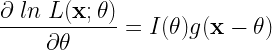
There exists an unbiased estimator that attains CRLB if and only if,
Here \( ln \; L(\mathbf{x};\theta) \) is the log likelihood function of x parameterized by \(\theta\) – the parameter to be estimated, \( I(\theta)\) is the Fisher Information and \( g(x)\) is some function.
Then, the estimator that attains CRLB is given by
Steps to find MVUE using CRLB:
If we could write the equation (as given above) in terms of Fisher Matrix and some function \( g(x)\) then \(g(x)\) is a Minimum Variable Unbiased Estimator.
1) Given a signal model \( x \), compute \(\frac{\partial\;ln\;L(\mathbf{x};\theta) }{\partial \theta }\)
2) Check if the above computation can be put in the form like the one given in the above theorem
3) Then \(g(\mathbf{x})\) given an MVUE
Let’s look at how CRLB can be used to find an MVUE for a signal that has a DC component embedded in AWGN noise.
Finding a MVUE to estimate DC component embedded in noise:
Consider the signal model where a DC component – \(A\) is embedded in an AWGN noise with zero mean and variance=\(\sigma \).
Our goal is to find an MVUE that could estimate the DC component from the observed samples \(x[n]\).
$$x[n] = A + w[n], \;\;\; n=0,1,2,\cdots,N-1 $$
We calculate CRLB and see if it can help us find a MVUE.
From the above equation we can readily identify \( I(A)\) and \(g(\mathbf{x})\) as follows
Thus,the Fisher Information \(I(A)\) and the MVUE \(g(\mathbf{x})\) are given by
Thus for a signal model which has a DC component in AWGN, the sample mean of observed samples \(x[n]\) gives a Minimum Variance Unbiased Estimator to estimate the DC component.
Key focus: Discuss scalar parameter estimation using CRLB. Estimate DC component from observed data in the presence of AWGN noise.
Consider a set of observed data samples and is the scalar parameter that is to be estimated from the observed samples. The accuracy of the estimate depends on how well the observed data is influenced by the parameter . The observed data is considered as a random data whose PDF is influenced by . The PDF describes the dependence of X on .
If the of PDF depends weakly on then the estimates will be poor.If the of PDF on depends strongly on then the estimates will be good.
As seen in the previous section, the curvature of the likelihood function (Fisher Information) is related to the concentration of PDF. More the curvature, more is the concentration of PDF, more will be accuracy of estimates. The Fisher Information is calculated from log likelihood function as,
Under the regularity condition that the score of the log likelihood function is zero,
1) Given a model for observed data samples – , write the log likelihood function as a function of –
2) Keep as fixed and take the second partial derivative of the log likelihood function with respect to parameter to be estimated –
3) If the result depends on , fix and take the expected value with respect to . This step can be skipped if the result does not depend on .
4) If the result depends on , then evaluate the result at specific values of
5) Take the reciprocal of the result and negate it.
Let’s see an example for scalar parameter estimation using CRLB.
Derivation of CRLB for an embedded DC component in AWGN Noise:
Here is a constant DC value that has to be estimated from the observed data samples and is the AWGN noise with zero mean and variance=.
Given the fact that the samples are influenced by the AWGN noise with zero mean and variance=, the likelihood function can be written as
The log likelihood function is formed as,
Taking the first partial derivative of log likelihood function with respect to A,
Computing the second partial derivative of log likelihood function by differentiating one more time,
The Fisher Information is given by taking the expectation and negating it.
The Cramér-Rao Lower Bound is the reciprocal of Fisher Information I(A)
The variance of any estimator that estimates the DC component from the given observed samples will always be greater that the CRLB. That is, the CRLB acts as the lower bound for the variance of the estimates. This can be conveniently represented as
Tweaking the CRLB:
Now that we have found an expression for CRLB for the estimation of the DC component, we can look for schemes that may affect the CRLB. From the expression of CRLB, following points can be inferred.
1) The CRLB does not depend on the parameter to be estimated ()
2) The CRLB increases linearly with
3) The CRLB decreases inversely with
Key concept: Cramér-Rao bound is the lower bound on variance of unbiased estimators that estimate deterministic parameters.
Introduction
The criteria for existence of having an Minimum Variance Unbiased Estimator (MVUE) was discussed in a previous article. To have an MVUE, it is necessary to have estimates that are unbiased and that give minimum variance (compared to the true parameter value). This is given by the following two equations
For a MVUE, it is easier to verify the first criteria (unbiased-ness) using the first equation, but verifying the second criteria (minimum variance) is tricky. We can only calculate the variance of the estimator, but how can we make sure that it is “the minimum”? How can we make sure that a designed estimator gives the minimum variance? There may exist other numerous unbiased estimators (which we may not know) that may give minimum variance. Other words, how do we make sure that our estimate is the best MVUE in the world? Cramér-Rao Lower Bound (CRLB) may come to our rescue.
Cramér-Rao Lower Bound (CRLB):
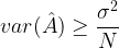
Harald Cramér and Radhakrishna Rao derived a way to express the lower bound on the variance of unbiased estimators that estimate deterministic parameters. This lower bound is called as the Cramér-Rao Lower Bound (CRLB).
If is an unbiased estimate of a deterministic parameter , then the relationship between the variance of the estimates ( ) and CRLB can be expressed as
CRLB tell us the best minimum variance that we can expect to get from an unbiased estimator.
Applications of CRLB include :
1) Making judgment on proposed estimators. Estimators whose variance is not close to CRLB are considered inferior. 2) To do feasibility studies as to whether a particular estimator/system can meet given specifications. It is also used to rule out impossible estimators – No estimator can beat CRLB (example: Figure 1). 3) Benchmark for comparing unbiased estimators. 4) It may sometimes provide MVUE. If an unbiased estimator achieved CRLB, it means that it is a MVUE.
Figure 1: CRLB and the efficient estimator for phase estimation
Feasibility Studies :
Derivation of CRLB for a particular given scenario or proposed algorithm of estimation is often found in research texts. The derived theoretical CRLB for a system/algorithm is compared with actual variance of the implemented system and conclusions are drawn. For example, in the paper titled “A Novel Frequency Synchronization Algorithm and its Cramer Rao Bound in Practical UWB Environment for MB-OFDM Systems”[1] – a frequency offset estimation algorithm was proposed for estimating frequency offsets in multi-band orthogonal frequency division multiplexing (MB-OFDM) systems. The performance of the algorithm was studied by BER analysis (Eb/N0 Vs BER curves). Additionally,the estimator performance is further validated by comparing the simulated estimator variance with the derived theoretical CRLB for four UWB channel models.
Rate this article: Note: There is a rating embedded within this post, please visit this post to rate it.
As we have seen in the previous articles, that the estimation of a parameter from a set of data samples depends strongly on the underlying PDF. The accuracy of the estimation is inversely proportional to the variance of the underlying PDF. That is, less the variance of PDF more is the accuracy of estimation and vice versa. In other words, the estimation accuracy depends on the sharpness of the PDF curve. Sharper the PDF curve more is the accuracy.
Gradient and score :
In geometry, given any curve, the gradient (also called slope) of the curve is zero at maximum and minimum points of the curve. Gradient of a function (representing a curve) is calculated by its first derivative. The gradient of log likelihood function is called score and is used to find Maximum Likelihood estimate of a parameter.
Figure: The gradient of log likelihood function is called score
Denoting the score as u(θ),
At the MLE point, where the true value of the parameter θ is equal to the ML estimate the gradient is zero. Thus equating the score to zero and finding the corresponding gives the ML estimate of θ (provided the log likelihood function is a concave curve).
Curvature and Fisher Information :
In geometry, the sharpness of a curve is measured by its Curvature. The sharpness of a PDF curve is influenced by its variance. More the variance less is the sharpness and vice versa. The accuracy of the estimator is measure by the sharpness of the underlying PDF curve. In differential geometry, the curvature is related to second derivative of a function.
The mean of the score evaluated at ML estimate (or true value of estimate) θ is zero. This gives,
Under this regularity condition that the expectation of the score is zero, the variance of the score is called Fisher Information. That is the expectation of second derivative of log likelihood function is called Fisher Information. It measures the sharpness of the log likelihood function. More the value of Fisher Information; more is the sharpness of the curve and vice versa. So if we can calculate the Fisher Information of a log likelihood function, then we can know more about the accuracy or sensitivity of the estimator with respect to the parameter to be estimated.
Figure 2: The variance of the score is called Fisher Information
The Fisher Information denoted by I(θ) is given by the variance of the score.
Here the ∗ operator indicates the operation of taking complex conjugate. The negative sign in the above equation is introduced to bring inverse relationship between variance and the Fisher Information (i.e. Fisher Information will be high for log likelihood functions that have low variance). As we can see from the above equation, that the Fisher Information is related to the second derivative (Curvature or Sharpness) of the log likelihood function. The I(θ) computed above is also called Observed Fisher Information.
Rate this article: Note: There is a rating embedded within this post, please visit this post to rate it.
Note: There is a rating embedded within this post, please visit this post to rate it.
As a pre-requisite, check out the previous article on the logic behind deriving the maximum likelihood estimator for a given PDF.
Let X=(x1,x2,…, xN) are the samples taken from Gaussian distribution given by
Calculating the Likelihood
The log likelihood is given by,
Differentiating and equating to zero to find the maxim (otherwise equating the score to zero)
Thus the mean of the samples gives the MLE of the parameter .
Note: There is a rating embedded within this post, please visit this post to rate it.
As a pre-requisite, check out the previous article on the logic behind deriving the maximum likelihood estimator for a given PDF.
Let X=(x1,x2,…, xN) are the samples taken from Exponential distribution given by
Calculating the Likelihood
The log likelihood is given by,
Differentiating and equating to zero to find the maxim (otherwise equating the score to zero)
Thus the inverse of mean of the samples gives the MLE of the parameter .
Note: There is a rating embedded within this post, please visit this post to rate it.
Suppose X=(x1,x2,…, xN) are the samples taken from a random distribution whose PDF is parameterized by the parameter . If the PDF of the underlying parameter satisfies some regularity condition (if the log of the PDF is differentiable) then the likelihood function is given by
Here is the PDF of the underlying distribution.
Hereafter we will denote as .
The maximum likelihood estimate of the unknown parameter can be found by selecting the say some for which the likelihood function attains maximum. We usually use log of the likelihood function to simplify multiplications into additions. So restating this, the maximum likelihood estimate of the unknown parameter can be found by selecting the say some for which the log likelihood function attains maximum.
In differential geometry, the maximum of a function f(x) is found by taking the first derivative of the function and equating it to zero. Similarly, the maximum likelihood estimate of a parameter – is found by partially differentiating the likelihood function or the log likelihood function and equating it to zero.
The first partial derivative of log likelihood function with respect to is also called score. The variance of the score (partial derivative of score with respect to ) is known as Fisher Information.
Calculating MLE for Poisson distribution:
Let X=(x1,x2,…, xN) are the samples taken from Poisson distribution given by
Calculating the Likelihood
The log likelihood is given by,
Differentiating and equating to zero to find the maxim (otherwise equating the score to zero)
Thus the mean of the samples gives the MLE of the parameter .
To be updated soon
For the derivation of other PDFs see the following links
Theoretical derivation of Maximum Likelihood Estimator for Exponential PDF
Theoretical derivation of Maximum Likelihood Estimator for Gaussian PDF
Key focus: Understand maximum likelihood estimation (MLE) using hands-on example. Know the importance of log likelihood function and its use in estimation problems.
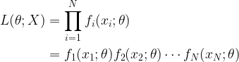
Likelihood Function:
Suppose X=(x1,x2,…, xN) are the samples taken from a random distribution whose PDF is parameterized by the parameter θ. The likelihood function is given by
Here fN(xN;θ) is the PDF of the underlying distribution.
The above equation differs significantly from the joint probability calculation that in joint probability calculation, θ is considered a random variable. In the above equation, the parameter θ is the parameter to be estimated.
Example:
Consider the DC estimation problem presented in the previous article where a transmitter transmits continuous stream of data samples representing a constant value – A. The data samples sent via a communication channel gets added with White Gaussian Noise – w[n] (with μ=0 and σ2=1 ). The receiver receives the samples and its goal is to estimate the actual DC component – A in the presence of noise.
Figure 1: The problem of DC estimation
Likelihood as an Estimation Metric:
Let’s use the likelihood function as estimation metric. The estimation of A depends on the PDF of the underlying noise-w[n]. The estimation accuracy depends on the variance of the noise. More the variance less is the accuracy of estimation and vice versa.
Let’s fix A=1.3 and generate 10 samples from the above model (Use the Matlab script given below to test this. You may get different set of numbers). Now we pretend that we do not know anything about the model and all we want to do is to estimate the DC component (Parameter to be estimated θ=A) from the observed samples:
Assuming a variance of 1 for the underlying PDF, we will try a range of values for A from -2.0 to +1.5 in steps of 0.1 and calculate the likelihood function for each value of A.
Matlab script:
% Demonstration of Maximum Likelihood Estimation in Matlab
%   Author: Mathuranathan (https://www.gaussianwaves.com)
%   License : creative commons : Attribution-NonCommercial-ShareAlike 3.0 Unported

A=1.3;
N=10; %Number of Samples to collect
x=A+randn(1,N);

s=1; %Assume standard deviation s=1

rangeA=-2:0.1:5; %Range of values of estimation parameter to test
L=zeros(1,length(rangeA)); %Place holder for likelihoods

for i=1:length(rangeA)
    %Calculate Likelihoods for each parameter value in the range
    L(i) = exp(-sum((x-rangeA(i)).^2)/(2*s^2));  %Neglect the constant term (1/(sqrt(2*pi)*sigma))^N as it will pull %down the likelihood value to zero for increasing value of N
end

[maxL,index]=max(L); %Select the parameter value with Maximum Likelihood
display('Maximum Likelihood of A');
display(rangeA(index));

%Plotting Commands
plot(rangeA,L);hold on;
stem(rangeA(index),L(index),'r'); %Point the Maximum Likelihood Estimate
displayText=['\leftarrow Likelihood of A=' num2str(rangeA(index))];
title('Maximum Likelihood Estimation of unknown Parameter A');
xlabel('\leftarrow A');
ylabel('Likelihood');
text(rangeA(index),L(index)/3,displayText,'HorizontalAlignment','left');

figure(2);
plot(rangeA,log(L));hold on;
YL = ylim;YMIN = YL(1);
plot([rangeA(index) rangeA(index)],[YMIN log(L(index))] ,'r'); %Point the Maximum Likelihood Estimate
title('Log Likelihood Function');
xlabel('\leftarrow A');
ylabel('Log Likelihood');
text([rangeA(index)],YMIN/2,displayText,'HorizontalAlignment','left');
Simulation Result:
For the above mentioned 10 samples of observation, the likelihood function over the range (-2:0.1:1.5) of DC component values is plotted below. The maximum likelihood value happens at A=1.4 as shown in the figure. The estimated value of A is 1.4 since the maximum value of likelihood occurs there.
This estimation technique based on maximum likelihood of a parameter is called Maximum Likelihood Estimation (MLE). The estimation accuracy will increase if the number of samples for observation is increased. Try the simulation with the number of samples N set to 5000 or 10000 and observe the estimated value of A for each run.
Figure 2: Maximum likelihood estimation of unknown parameter A
Log Likelihood Function:
It is often useful to calculate the log likelihood function as it reduces the above mentioned equation to series of additions instead of multiplication of several terms. This is particularly useful when implementing the likelihood metric in digital signal processors. The log likelihood is simply calculated by taking the logarithm of the above mentioned equation. The decision is again based on the maximum likelihood criterion.
Figure 3: Maximum likelihood estimation using log likelihood function
Advantages of Maximum Likelihood Estimation:
* Asymptotically Efficient – meaning that the estimate gets better with more samples * Asymptotically unbiased * Asymptotically consistent * Easier to compute * Estimation without any prior information * The estimates closely agree with the data
Disadvantages of Maximum Likelihood Estimation:
* Since the estimates closely agree with data, it will give noisy estimates for data mixed with noise. * It does not utilize any prior information for the estimation. But in real world scenario, we always have some prior information about the parameter to be estimated. We should always use it to our advantage despite it introducing bias in the estimates.
Rate this article: Note: There is a rating embedded within this post, please visit this post to rate it.
Estimator bias: Systematic deviation from the true value, either consistently overestimating or underestimating the parameter of interest.
Estimator Bias: Biased or Unbiased
Consider a simple communication system model where a transmitter transmits continuous stream of data samples representing a constant value – ‘A’. The data samples sent via a communication channel gets added with White Gaussian Noise – ‘w[n]’ (with mean=0 and variance=1). The receiver receives the samples and its goal is to estimate the actual constant value (we will call it DC component hereafter) transmitted by the transmitter in the presence of noise. This is a classical DC estimation problem.
Since the constant DC component is embedded in noise, we need to come up with an estimator function to estimate the DC component from the received samples. The goal of our estimator function is to estimate the DC component so that the mean of the estimate should be equal to the actual DC value. This is the criteria for ascertaining the unbiased-ness of an estimator.
The following figure captures the difference between a biased estimator and an unbiased estimator.
Example for understanding estimator bias
Consider that we are presented with a set of N samples of data representing x[n] at the receiver. Let’s us take the signal model that represents the received data samples :
Consider two estimator models/functions to estimate the DC component from the received samples. We will see which of the two estimator functions gives us unbiased estimate.
\( \begin{align} &= A; if \; A=0 \\ & \neq A; if \; A \neq 0 \end{align} \)
Bias
Unbiased
Biased
Testing the bias of an estimation in Matlab:
To test the bias of the above mentioned estimators in Matlab, the signal model: \(x[n]=A+w[n]\) is taken as a starting point. Here \(A\) is a constant DC value (say for example it takes a value of 1.5) and w[n] is a vector of random noise that follows standard normal distribution with mean=0 and variance=1.
Generate 5000 signal samples \(x[n]\) by setting \(A=1.5\) and adding it with \(w[n]\) generated using Matlab’s “randn” function.
N=5000; %Number of samples for the test
A=1.5 ;%Actual DC value
w = randn(1,N); %Standard Normal Distribution mean=0,variance=1 represents noise
x = A + w ;  %Received signal samples
Implement the above mentioned estimator functions and display their estimated values
estA1 = sum(x)/N;%  Estimated DC component from x[n] using estimator 1
estA2 = sum(x)/(2*N); %  Estimated DC component from x[n] using estimator 2

%Display estimated values
disp([‘Estimator 1: ’ num2str(estA1) ]);
disp([‘Estimator 2: ’ num2str(estA2) ]);
Sample Result :
Estimator 1: 1.5185 % Estimator 1’s result will near exact value of 1.5 as N grows larger
Estimator 2: 0.75923 % Estimator 2’s result is biased as it is far away from the actual DC value
The above result just prints the estimated value. Since the estimated parameter – \(\hat{A}\) is a constant \(E(\hat{A}) = \hat{A}\). In real world scenario, the parameter that is estimated, will be a random variable. In that case you have to print the “expectation” (mean) of the estimated value for comparison.
This website uses cookies to improve your experience while you navigate through the website. Out of these, the cookies that are categorized as necessary are stored on your browser as they are essential for the working of basic functionalities of the website. We also use third-party cookies that help us analyze and understand how you use this website. These cookies will be stored in your browser only with your consent. You also have the option to opt-out of these cookies. But opting out of some of these cookies may affect your browsing experience.
Necessary cookies are absolutely essential for the website to function properly. These cookies ensure basic functionalities and security features of the website, anonymously.
Cookie
Duration
Description
cookielawinfo-checbox-analytics
11 months
This cookie is set by GDPR Cookie Consent plugin. The cookie is used to store the user consent for the cookies in the category "Analytics".
cookielawinfo-checbox-analytics
11 months
This cookie is set by GDPR Cookie Consent plugin. The cookie is used to store the user consent for the cookies in the category "Analytics".
cookielawinfo-checbox-functional
11 months
The cookie is set by GDPR cookie consent to record the user consent for the cookies in the category "Functional".
cookielawinfo-checbox-functional
11 months
The cookie is set by GDPR cookie consent to record the user consent for the cookies in the category "Functional".
cookielawinfo-checbox-others
11 months
This cookie is set by GDPR Cookie Consent plugin. The cookie is used to store the user consent for the cookies in the category "Other.
cookielawinfo-checbox-others
11 months
This cookie is set by GDPR Cookie Consent plugin. The cookie is used to store the user consent for the cookies in the category "Other.
cookielawinfo-checkbox-necessary
11 months
This cookie is set by GDPR Cookie Consent plugin. The cookies is used to store the user consent for the cookies in the category "Necessary".
cookielawinfo-checkbox-performance
11 months
This cookie is set by GDPR Cookie Consent plugin. The cookie is used to store the user consent for the cookies in the category "Performance".
viewed_cookie_policy
11 months
The cookie is set by the GDPR Cookie Consent plugin and is used to store whether or not user has consented to the use of cookies. It does not store any personal data.
Functional cookies help to perform certain functionalities like sharing the content of the website on social media platforms, collect feedbacks, and other third-party features.
Performance cookies are used to understand and analyze the key performance indexes of the website which helps in delivering a better user experience for the visitors.
Analytical cookies are used to understand how visitors interact with the website. These cookies help provide information on metrics the number of visitors, bounce rate, traffic source, etc.


![I(\theta) = -E\left [ \frac{\partial^2 ln L(\theta)}{\partial \theta^2} \right ]](https://s0.wp.com/latex.php?latex=I%28%5Ctheta%29+%3D+-E%5Cleft+%5B+%5Cfrac%7B%5Cpartial%5E2+ln+L%28%5Ctheta%29%7D%7B%5Cpartial+%5Ctheta%5E2%7D+%5Cright+%5D+&bg=ffffff&fg=000&s=2&c=20201002)

![E\left [ \frac{\partial ln L(\theta) }{\partial \theta } \right ] = 0 \;\;\; \forall\theta](https://s0.wp.com/latex.php?latex=E%5Cleft+%5B+%5Cfrac%7B%5Cpartial+ln+L%28%5Ctheta%29+%7D%7B%5Cpartial+%5Ctheta+%7D+%5Cright+%5D+%3D+0+%5C%3B%5C%3B%5C%3B+%5Cforall%5Ctheta+&bg=ffffff&fg=000&s=2&c=20201002)


![\text{Data Model: } x[n] = A + w[n], \;\;\; n=0,1,2,\cdots,N-1](https://s0.wp.com/latex.php?latex=%5Ctext%7BData+Model%3A+%7D+x%5Bn%5D+%3D+A+%2B+w%5Bn%5D%2C+%5C%3B%5C%3B%5C%3B+n%3D0%2C1%2C2%2C%5Ccdots%2CN-1%C2%A0+&bg=ffffff&fg=000&s=2&c=20201002)


![x[n]](https://s0.wp.com/latex.php?latex=x%5Bn%5D&bg=ffffff&fg=000&s=0&c=20201002)

![w[n]](https://s0.wp.com/latex.php?latex=w%5Bn%5D&bg=ffffff&fg=000&s=0&c=20201002)


![\displaystyle{ln\;L(x;A) =-\frac{N}{2}ln(2\pi\sigma^2) - \frac{1}{2\sigma^2}\sum_{n=0}^{N-1}(x[n]-A)^2}](https://s0.wp.com/latex.php?latex=%5Cdisplaystyle%7Bln%5C%3BL%28x%3BA%29+%3D-%5Cfrac%7BN%7D%7B2%7Dln%282%5Cpi%5Csigma%5E2%29+-+%5Cfrac%7B1%7D%7B2%5Csigma%5E2%7D%5Csum_%7Bn%3D0%7D%5E%7BN-1%7D%28x%5Bn%5D-A%29%5E2%7D+&bg=ffffff&fg=000&s=2&c=20201002)


![\sigma^{2}_{ \hat{f}_0 }=E \left\{ \left( \hat{f}_0 - E [ \hat{f}_0 ] \right)^2 \right\} \quad \text{should be minimum}](https://s0.wp.com/latex.php?latex=%5Csigma%5E%7B2%7D_%7B+%5Chat%7Bf%7D_0+%7D%3DE+%5Cleft%5C%7B+%5Cleft%28+%5Chat%7Bf%7D_0+-+E+%5B+%5Chat%7Bf%7D_0+%5D++%5Cright%29%5E2+%5Cright%5C%7D+%5Cquad+%5Ctext%7Bshould+be+minimum%7D+&bg=ffffff&fg=000&s=2&c=20201002)


![u(\theta) =\frac{\partial }{\partial \theta} \left[ ln L(\theta) \right ]](https://s0.wp.com/latex.php?latex=u%28%5Ctheta%29+%3D%5Cfrac%7B%5Cpartial+%7D%7B%5Cpartial+%5Ctheta%7D+%5Cleft%5B+ln+L%28%5Ctheta%29+%5Cright+%5D+&bg=ffffff&fg=000&s=1&c=20201002)


![E[u(\theta)] = 0](https://s0.wp.com/latex.php?latex=E%5Bu%28%5Ctheta%29%5D+%3D+0+&bg=ffffff&fg=000&s=1&c=20201002)


![\displaystyle{\begin{aligned} I(\theta) &= -var \left[ u (\theta) \right] \\ &= - E \left[ u (\theta) u^\ast (\theta) \right] \\ &= - E \left[ \frac{\partial^2 \; ln \left[ L(\theta) \right] }{\partial \theta^2} \right] \end{aligned}}](https://s0.wp.com/latex.php?latex=%5Cdisplaystyle%7B%5Cbegin%7Baligned%7D+I%28%5Ctheta%29+%26%3D+-var+%5Cleft%5B+u+%28%5Ctheta%29+%5Cright%5D+%5C%5C+%26%3D+-+E+%5Cleft%5B+u+%28%5Ctheta%29+u%5E%5Cast+%28%5Ctheta%29+%5Cright%5D+%5C%5C+%26%3D+-+E+%5Cleft%5B+%5Cfrac%7B%5Cpartial%5E2+%5C%3B+ln+%5Cleft%5B+L%28%5Ctheta%29+%5Cright%5D+%7D%7B%5Cpartial+%5Ctheta%5E2%7D+%5Cright%5D+%5Cend%7Baligned%7D%7D+&bg=ffffff&fg=000&s=1&c=20201002)