Auto-correlation, also called series correlation, is the correlation of a given sequence with itself as a function of time lag. Cross-correlation is a more generic term, which gives the correlation between two different sequences as a function of time lag.
Given two sequences


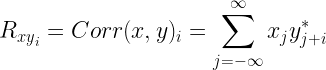
Auto-correlation is a special case of cross-correlation, where x=y. One can use a brute force method (using for loops implementing the above equation) to compute the auto-correlation sequence. However, other alternatives are also at your disposal.
Method 1: Auto-correlation using xcorr function
Matlab
For a N-dimensional given vector x, the Matlab command xcorr(x,x) or simply xcorr(x) gives the auto-correlation sequence. For the input sequence x=[1,2,3,4], the command xcorr(x) gives the following result.
>> x=[1 2 3 4]
>> acf=xcorr(x)
acf= 4   11   20   30   20   11  4
Python
In Python, autocorrelation of 1-D sequence can be obtained using numpy.correlate function. Set the parameter mode=’full’ which is useful for calculating the autocorrelation as a function of lag.
import numpy as np
x = np.asarray([1,2,3,4])
np.correlate(x, x,mode='full')
# output: array([ 4, 11, 20, 30, 20, 11,  4])
Method 2: Auto-correlation using Convolution
Auto-correlation sequence can be computed as the convolution between the given sequence and the reversed (flipped) version of the conjugate of the sequence.The conjugate operation is not needed if the input sequence is real.
Matlab
>> x=[1 2 3 4]
>> acf=conv(x,fliplr(conj(x)))
acf= 4   11   20   30   20   11  4
Python
import numpy as np
x = np.asarray([1,2,3,4])
np.convolve(x,np.conj(x)[::-1])
# output: array([ 4, 11, 20, 30, 20, 11,  4])
Method 3: Autocorrelation using Toeplitz matrix
Autocorrelation sequence can be found using Toeplitz matrices. An example for using Toeplitz matrix structure for computing convolution is given here. The same technique is extended here, where one signal is set as input sequence and the other is just the flipped version of its conjugate. The conjugate operation is not needed if the input sequence is real.
Matlab
>> x=[1 2 3 4]
>> acf=toeplitz([x zeros(1,length(x)-1)],[x(1) zeros(1,length(conj(x))-1)])*fliplr(x).'
acf= 4   11   20   30   20   11  4
Python
import numpy as np
from scipy.linalg import toeplitz
x = np.asarray([1,2,3,4])
toeplitz(np.pad(x, (0,len(x)-1),mode='constant'),np.pad([x[0]], (0,len(x)-1),mode='constant'))@x[::-1]
# output: array([ 4, 11, 20, 30, 20, 11, 4])
Method 4: Auto-correlation using FFT/IFFT
Auto-correlation sequence can be found using FFT/IFFT pairs. An example for using FFT/IFFT for computing convolution is given here. The same technique is extended here, where one signal is set as input sequence and the other is just the flipped version of its conjugate.The conjugate operation is not needed if the input sequence is real.
Matlab
>> x=[1 2 3 4]
>> L = 2*length(x)-1
>> acf=ifft(fft(x,L).*fft(fliplr(conj(x)),L))
acf= 4   11   20   30   20   11  4
Python
import numpy as np
from scipy.fftpack import fft,ifft

x = np.asarray([1,2,3,4])

L = 2*len(x) - 1
ifft(fft(x,L)*fft(np.conj(x)[::-1],L))
#output: array([ 4+0j, 11+0j, 20+0j, 30+0j, 20+0j, 11+0j, 4+0j])
Note that in all the above cases, due to the symmetry property of auto-correlation function, the center element represents


Construction the Auto-correlation Matrix
Auto-correlation matrix is a special form of matrix constructed from auto-correlation sequence. It takes the following form.

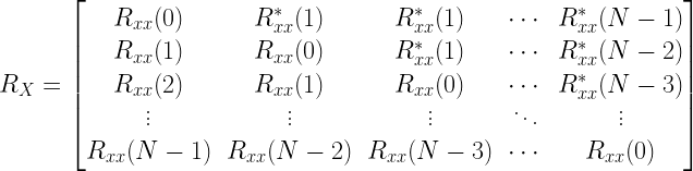
The auto-correlation matrix is easily constructed, once the auto-correlation sequence


Matlab
>> x=[1+j 2+j 3-j] %x is complex
>> acf=conv(x,fliplr(conj(x)))% %using Method 2 to compute Auto-correlation sequence
>>Rxx=acf(3:end); % R_xx(0) is the center element
>>Rx=toeplitz(Rxx,[Rxx(1) conj(Rxx(2:end))])
Python
import numpy as np
x = np.asarray([1+1j,2+1j,3-1j]) #x is complex
acf = np.convolve(x,np.conj(x)[::-1]) # using Method 2 to compute Auto-correlation sequence
Rxx=acf[2:]; # R_xx(0) is the center element
Rx = toeplitz(Rxx,np.hstack((Rxx[0], np.conj(Rxx[1:]))))
Result:


Rate this article: Note: There is a rating embedded within this post, please visit this post to rate it.
References:
[1] Reddi.S.S,”Eigen Vector properties of Toeplitz matrices and their application to spectral analysis of time series, Signal Processing, Vol 7,North-Holland, 1984,pp 46-56.↗
[2] Robert M. Gray,”Toeplitz and circulant matrices – an overview”,Department of Electrical Engineering,Stanford University,Stanford 94305,USA.↗
[3] Matlab documentation help on Toeplitz command.↗
Books by the author
 Wireless Communication Systems in Matlab Second Edition(PDF) Note: There is a rating embedded within this post, please visit this post to rate it. |  Digital Modulations using Python (PDF ebook) Note: There is a rating embedded within this post, please visit this post to rate it. |  Digital Modulations using Matlab (PDF ebook) Note: There is a rating embedded within this post, please visit this post to rate it. |
| Hand-picked Best books on Communication Engineering Best books on Signal Processing |
||


![a=[a_0,a_1,a_2,...,a_{n-1}]](https://s0.wp.com/latex.php?latex=a%3D%5Ba_0%2Ca_1%2Ca_2%2C...%2Ca_%7Bn-1%7D%5D&bg=ffffff&fg=000&s=0&c=20201002)

![a=[a_0,a_1,a_2,...,a_n]](https://s0.wp.com/latex.php?latex=a%3D%5Ba_0%2Ca_1%2Ca_2%2C...%2Ca_n%5D&bg=ffffff&fg=000&s=0&c=20201002)

![b=[b_0,b_1,b_2,...,b_n]](https://s0.wp.com/latex.php?latex=b%3D%5Bb_0%2Cb_1%2Cb_2%2C...%2Cb_n%5D&bg=ffffff&fg=000&s=0&c=20201002)


![p(x) . q(x)=(p\ast q)(x)=a.b=[c_0,c_1,c_2,\cdots,c_{n+m}] \; , \;where](https://s0.wp.com/latex.php?latex=p%28x%29+.+q%28x%29%3D%28p%5Cast+q%29%28x%29%3Da.b%3D%5Bc_0%2Cc_1%2Cc_2%2C%5Ccdots%2Cc_%7Bn%2Bm%7D%5D+%5C%3B+%2C+%5C%3Bwhere+&bg=ffffff&fg=000&s=2&c=20201002)


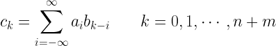

![c[k]=\displaystyle{\sum_{i=-\infty}^{\infty}a[i]b[k-i]} \quad\quad k=0,1,\cdots,n+m](https://s0.wp.com/latex.php?latex=c%5Bk%5D%3D%5Cdisplaystyle%7B%5Csum_%7Bi%3D-%5Cinfty%7D%5E%7B%5Cinfty%7Da%5Bi%5Db%5Bk-i%5D%7D+%5Cquad%5Cquad+k%3D0%2C1%2C%5Ccdots%2Cn%2Bm+&bg=ffffff&fg=000&s=2&c=20201002)


![h[n]](https://s0.wp.com/latex.php?latex=h%5Bn%5D&bg=ffffff&fg=000&s=0&c=20201002)
![x[n]](https://s0.wp.com/latex.php?latex=x%5Bn%5D&bg=ffffff&fg=000&s=0&c=20201002)

![y[n]](https://s0.wp.com/latex.php?latex=y%5Bn%5D&bg=ffffff&fg=000&s=0&c=20201002)

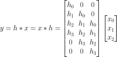
![y[k]=h[n]*x[n] = \displaystyle{\sum_{i=-\infty}^{\infty}x[i]h[k-i]}](https://s0.wp.com/latex.php?latex=y%5Bk%5D%3Dh%5Bn%5D%2Ax%5Bn%5D+%3D+%5Cdisplaystyle%7B%5Csum_%7Bi%3D-%5Cinfty%7D%5E%7B%5Cinfty%7Dx%5Bi%5Dh%5Bk-i%5D%7D+&bg=ffffff&fg=000&s=2&c=20201002)

![h[n]=[h_0,h_1,h_2,h_3]](https://s0.wp.com/latex.php?latex=h%5Bn%5D%3D%5Bh_0%2Ch_1%2Ch_2%2Ch_3%5D&bg=ffffff&fg=000&s=0&c=20201002)

![x[n]=[x_0,x_1,x_2]](https://s0.wp.com/latex.php?latex=x%5Bn%5D%3D%5Bx_0%2Cx_1%2Cx_2%5D&bg=ffffff&fg=000&s=0&c=20201002)

![h[n] \ast x[n]](https://s0.wp.com/latex.php?latex=h%5Bn%5D+%5Cast+x%5Bn%5D&bg=ffffff&fg=000&s=0&c=20201002)

![y[k]=h[n]*x[n] = \displaystyle{\sum_{i=-\infty}^{\infty}x[i]h[k-i]} \quad k=0,1,\cdots,5](https://s0.wp.com/latex.php?latex=y%5Bk%5D%3Dh%5Bn%5D%2Ax%5Bn%5D+%3D+%5Cdisplaystyle%7B%5Csum_%7Bi%3D-%5Cinfty%7D%5E%7B%5Cinfty%7Dx%5Bi%5Dh%5Bk-i%5D%7D+%5Cquad+k%3D0%2C1%2C%5Ccdots%2C5+&bg=ffffff&fg=000&s=2&c=20201002)


![\begin{bmatrix} y[0]\\y[1]\\y[2]\\y[3]\\y[4]\\y[5] \end{bmatrix}=\begin{bmatrix}h[0] &0 & 0 \\ h[1] & h[0] & 0 \\ h[2] & h[1] & h[0] \\ h[3] & h[2] & h[1] \\ 0 & h[3] & h[2] \\ 0 & 0 & h[3] \end{bmatrix} \begin{bmatrix}x[0]\\x[1]\\x[2] \end{bmatrix}](https://s0.wp.com/latex.php?latex=%5Cbegin%7Bbmatrix%7D+y%5B0%5D%5C%5Cy%5B1%5D%5C%5Cy%5B2%5D%5C%5Cy%5B3%5D%5C%5Cy%5B4%5D%5C%5Cy%5B5%5D+%5Cend%7Bbmatrix%7D%3D%5Cbegin%7Bbmatrix%7Dh%5B0%5D+%260+%26+0+%5C%5C+h%5B1%5D+%26+h%5B0%5D+%26+0+%5C%5C+h%5B2%5D+%26+h%5B1%5D+%26+h%5B0%5D+%5C%5C+h%5B3%5D+%26+h%5B2%5D+%26+h%5B1%5D+%5C%5C+0+%26+h%5B3%5D+%26+h%5B2%5D+%5C%5C+0+%26+0+%26+h%5B3%5D+%5Cend%7Bbmatrix%7D+%5Cbegin%7Bbmatrix%7Dx%5B0%5D%5C%5Cx%5B1%5D%5C%5Cx%5B2%5D+%5Cend%7Bbmatrix%7D+&bg=ffffff&fg=000&s=2&c=20201002)


![X[z]](https://s0.wp.com/latex.php?latex=X%5Bz%5D&bg=ffffff&fg=000&s=0&c=20201002)


