Key focus: Know how to generate a gaussian pulse, compute its Fourier Transform using FFT and power spectral density (PSD) in Matlab & Python.
Numerous texts are available to explain the basics of Discrete Fourier Transform and its very efficient implementation – Fast Fourier Transform (FFT). Often we are confronted with the need to generate simple, standard signals (sine, cosine, Gaussian pulse, squarewave, isolated rectangular pulse, exponential decay, chirp signal) for simulation purpose. I intend to show (in a series of articles) how these basic signals can be generated in Matlab and how to represent them in frequency domain using FFT.
This article is part of the following books |
Gaussian Pulse : Mathematical description:
In digital communications, Gaussian Filters are employed in Gaussian Minimum Shift Keying – GMSK (used in GSM technology) and Gaussian Frequency Shift Keying (GFSK). Two dimensional Gaussian Filters are used in Image processing to produce Gaussian blurs. The impulse response of a Gaussian Filter is Gaussian. Gaussian Filters give no overshoot with minimal rise and fall time when excited with a step function. Gaussian Filter has minimum group delay. The impulse response of a Gaussian Filter is written as a Gaussian Function as follows

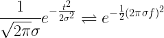
The Fourier Transform of a Gaussian pulse preserves its shape.
![\begin{aligned} G(f) &=F[g(t)]\\ &= \int_{-\infty }^{\infty } g(t)e^{-j2\pi ft}\, dt\\ &= \frac{1}{\sigma \sqrt{2 \pi } } \int_{-\infty }^{\infty } e^{- \frac{t^2}{2 \sigma^2}}e^{-j2\pi ft}\, dt\\ &=\frac{1}{\sigma \sqrt{2 \pi } } \int_{-\infty }^{\infty } e^{- \frac{1}{2 \sigma^2}\left[t^2+j4 \pi \sigma^2 ft \right]}\, dt\\ &=\frac{1}{\sigma \sqrt{2 \pi } } \int_{-\infty }^{\infty } e^{- \frac{1}{2 \sigma^2}\left[t^2+j4 \pi \sigma^2 ft + (j 2 \pi \sigma^2 f)^2 - (j 2 \pi \sigma^2 f)^2\right]}\, dt\\ &=e^{ \frac{1}{2 \sigma^2}(j 2 \pi \sigma^2 f)^2}\frac{1}{\sigma \sqrt{2 \pi } } \int_{-\infty }^{\infty } e^{- \frac{1}{2 \sigma^2}\left[t+j 2 \pi \sigma^2 f \right]^2}\, dt\\ &=e^{ \frac{1}{2 \sigma^2}(j 2 \pi \sigma^2 f)^2}=e^{ - \frac{1}{2}( 2 \pi \sigma f)^2}\end{aligned}](https://s0.wp.com/latex.php?latex=%5Cbegin%7Baligned%7D+G%28f%29+%26%3DF%5Bg%28t%29%5D%5C%5C+%26%3D+%5Cint_%7B-%5Cinfty+%7D%5E%7B%5Cinfty+%7D+g%28t%29e%5E%7B-j2%5Cpi+ft%7D%5C%2C+dt%5C%5C+%26%3D+%5Cfrac%7B1%7D%7B%5Csigma+%5Csqrt%7B2+%5Cpi+%7D+%7D+%5Cint_%7B-%5Cinfty+%7D%5E%7B%5Cinfty+%7D+e%5E%7B-+%5Cfrac%7Bt%5E2%7D%7B2+%5Csigma%5E2%7D%7De%5E%7B-j2%5Cpi+ft%7D%5C%2C+dt%5C%5C+%26%3D%5Cfrac%7B1%7D%7B%5Csigma+%5Csqrt%7B2+%5Cpi+%7D+%7D+%5Cint_%7B-%5Cinfty+%7D%5E%7B%5Cinfty+%7D+e%5E%7B-+%5Cfrac%7B1%7D%7B2+%5Csigma%5E2%7D%5Cleft%5Bt%5E2%2Bj4+%5Cpi+%5Csigma%5E2+ft+%5Cright%5D%7D%5C%2C+dt%5C%5C+%26%3D%5Cfrac%7B1%7D%7B%5Csigma+%5Csqrt%7B2+%5Cpi+%7D+%7D+%5Cint_%7B-%5Cinfty+%7D%5E%7B%5Cinfty+%7D+e%5E%7B-+%5Cfrac%7B1%7D%7B2+%5Csigma%5E2%7D%5Cleft%5Bt%5E2%2Bj4+%5Cpi+%5Csigma%5E2+ft+%2B+%28j+2+%5Cpi+%5Csigma%5E2+f%29%5E2+-+%28j+2+%5Cpi+%5Csigma%5E2+f%29%5E2%5Cright%5D%7D%5C%2C+dt%5C%5C+%26%3De%5E%7B+%5Cfrac%7B1%7D%7B2+%5Csigma%5E2%7D%28j+2+%5Cpi+%5Csigma%5E2+f%29%5E2%7D%5Cfrac%7B1%7D%7B%5Csigma+%5Csqrt%7B2+%5Cpi+%7D+%7D+%5Cint_%7B-%5Cinfty+%7D%5E%7B%5Cinfty+%7D+e%5E%7B-+%5Cfrac%7B1%7D%7B2+%5Csigma%5E2%7D%5Cleft%5Bt%2Bj+2+%5Cpi+%5Csigma%5E2+f+%5Cright%5D%5E2%7D%5C%2C+dt%5C%5C+%26%3De%5E%7B+%5Cfrac%7B1%7D%7B2+%5Csigma%5E2%7D%28j+2+%5Cpi+%5Csigma%5E2+f%29%5E2%7D%3De%5E%7B+-+%5Cfrac%7B1%7D%7B2%7D%28+2+%5Cpi+%5Csigma+f%29%5E2%7D%5Cend%7Baligned%7D+&bg=ffffff&fg=000&s=2&c=20201002)
The above derivation makes use of the following result from complex analysis theory and the property of Gaussian function – total area under Gaussian function integrates to 1.
By change of variable, let ( ).
).
![\displaystyle{\frac{1}{\sigma \sqrt{2 \pi} }\int_{-\infty }^{\infty }e^{- \frac{1}{2 \sigma^2}\left[t+j 2 \pi \sigma^2 f \right]^2}\, dt =\frac{1}{\sigma \sqrt{2 \pi } }\int_{-\infty }^{\infty }e^{- \frac{1}{2 \sigma^2} u^2}\, du =1}](https://s0.wp.com/latex.php?latex=%5Cdisplaystyle%7B%5Cfrac%7B1%7D%7B%5Csigma+%5Csqrt%7B2+%5Cpi%7D+%7D%5Cint_%7B-%5Cinfty+%7D%5E%7B%5Cinfty+%7De%5E%7B-+%5Cfrac%7B1%7D%7B2+%5Csigma%5E2%7D%5Cleft%5Bt%2Bj+2+%5Cpi+%5Csigma%5E2+f+%5Cright%5D%5E2%7D%5C%2C+dt+%3D%5Cfrac%7B1%7D%7B%5Csigma+%5Csqrt%7B2+%5Cpi+%7D+%7D%5Cint_%7B-%5Cinfty+%7D%5E%7B%5Cinfty+%7De%5E%7B-+%5Cfrac%7B1%7D%7B2+%5Csigma%5E2%7D+u%5E2%7D%5C%2C+du+%3D1%7D+&bg=ffffff&fg=000&s=2&c=20201002)
Thus, the Fourier Transform of a Gaussian pulse is a Gaussian Pulse.
Gaussian Pulse – Fourier Transform using FFT (Matlab & Python):
The following code generates a Gaussian Pulse with (  ). The Discrete Fourier Transform of this digitized version of Gaussian Pulse is plotted with the help of (FFT) function in Matlab.
For Python code, please refer the book Digital Modulations using Python
fs=80; %sampling frequency
sigma=0.1;
t=-0.5:1/fs:0.5; %time base

variance=sigma^2;
x=1/(sqrt(2*pi*variance))*(exp(-t.^2/(2*variance)));
subplot(2,1,1)
plot(t,x,'b');
title(['Gaussian Pulse \sigma=', num2str(sigma),'s']);
xlabel('Time(s)');
ylabel('Amplitude');

L=length(x);
NFFT = 1024;
X = fftshift(fft(x,NFFT));
Pxx=X.*conj(X)/(NFFT*NFFT); %computing power with proper scaling
f = fs*(-NFFT/2:NFFT/2-1)/NFFT; %Frequency Vector

subplot(2,1,2)
plot(f,abs(X)/fs,'r');
title('Magnitude of FFT');
xlabel('Frequency (Hz)')
ylabel('Magnitude |X(f)|');
xlim([-10 10])
Double Sided and Single Power Spectral Density using FFT:
Next, the Power Spectral Density (PSD) of the Gaussian pulse is constructed using the FFT. PSD describes the power contained at each frequency component of the given signal. Double Sided power spectral density is plotted first, followed by single sided power spectral density plot (retaining only the positive frequency side of the spectrum).
Pxx=X.*conj(X)/(L*L); %computing power with proper scaling
figure;
plot(f,10*log10(Pxx),'r');
title('Double Sided - Power Spectral Density');
xlabel('Frequency (Hz)')
ylabel('Power Spectral Density- P_{xx} dB/Hz');
X = fft(x,NFFT);
X = X(1:NFFT/2+1);%Throw the samples after NFFT/2 for single sided plot
Pxx=X.*conj(X)/(L*L);
f = fs*(0:NFFT/2)/NFFT; %Frequency Vector
figure;
plot(f,10*log10(Pxx),'r');
title('Single Sided - Power Spectral Density');
xlabel('Frequency (Hz)')
ylabel('Power Spectral Density- P_{xx} dB/Hz');
For Python code, please refer the book Digital Modulations using Python
Rate this article: 

 (13 votes, average: 3.85 out of 5)
Topics in this chapter
Books by the author
 Wireless Communication Systems in Matlab Second Edition(PDF) Note: There is a rating embedded within this post, please visit this post to rate it. |  Digital Modulations using Python (PDF ebook) Note: There is a rating embedded within this post, please visit this post to rate it. |  Digital Modulations using Matlab (PDF ebook) Note: There is a rating embedded within this post, please visit this post to rate it. |
| Hand-picked Best books on Communication Engineering Best books on Signal Processing |
||
I am sorry, correct link is actually https://dsp.stackexchange.com/a/87864/62232
Hey! Take a look on my post, There is a huge overlap in our question. There I also plotted the DFT and the DTFT.
https://dsp.stackexchange.com/a/85214/62232
Sorry, my previous suggestion is wrong.
It should be:
“plot(f,abs(X)/fs,’r’);”
Then G(0)=1 for all sigmas and all sample frequencies.
Peter
Hello Peter, Thanks for the suggestion. I have incorporate it in the code.
Mathuranathan
Hi Mathuranathan,
I think the line “plot(f,abs(X)/(L),’r’);” in the code is not correct. According to the equations, at the frequency f=0 the magnitude of G(0) is equal to 1. But the result of the code is 0.9877.
I think the correct line is:
“plot(f,abs(X)/(L-1),’r’);”
Note: (L) -> (L-1)
Kind regards from Germany,
Peter
Hello Peter,
Thanks for catching the mistake. I have corrected it.
Mathuranathan
Hi, thanks again for your works here.
I have a problem, I’m plotting a 3D Gaussian pulse.
I have been able to create it and to make the fft of it, but the phase it’s not null and quite incomprehensible.
This is a quick example of what I get:
close all;
clear;
clc;
N = 64; % Size of a sunction
D = N/2; % to indicate origin at the center of the function
a = 8; % radius for cylindrical function
w = 0.4; % decay rate for exponential function
y = repmat(1:N,N,1);
x = y’;
r = sqrt((D-x).^2+(D-y).^2); % definition of radius
sig = 5; % Variance for gaussian function
g = (2*pi*sig^2)*exp(-((r.^2))./(2*sig^2));
figure;mesh(g); title(‘2D Gaussian Function’);
G = fft2(g);
G = fftshift(G);
figure; mesh(abs(G)); title(‘Fourier Transform of Gaussian function’);
fzf=atan2(imag(G),real(G));
figure;
mesh(fzf);
title(‘Fourier Phase of Gaussian function’);
Never looked into the phase of a 3D gaussian pulse. So, I am not sure about the expected output.
Usage of atan2 could give spurious results as demonstrated here.
http://www.gaussianwaves.com/2015/11/interpreting-fft-results-obtaining-magnitude-and-phase-information/
The solution to the noisy phase spectrum is also given in the above link
Dear sir, this code is great for generating the gaussian pulse without using matlab toolboxes.
I want to ask that from the same code, if i want to generate the train of gaussian pulses, how can i generate (without using the matlab function pulstran)? kindly provide the baisc code for it. I have searched over the internet but not found. suppose I want to generate 12 gaussian pulses wtith sum time duration between them. plzz.
Hello this is Lingaraj, doing m-tech in belgaum. I have a problem in finding power spectral density using time domain approach,i have a written code found somewhere but i am not getting it. Please leave a reply as soon as possible…
Hi Viswanathan,
This really awesome article on Gaussian wave generation and analysis. I am trying to generate a Gaussian pulse of 20ns and plot the frequency response of it. When I try to simulate it in matlab, it gives me error saying out of memory. I think I am doing something wrong with the code:
function [ output_args ] = freqencySpectrum( ~ )
fs=0.00000001; // sampling at twice the highest frequency (20ns =50MHz, so sampling at 100MHz)
t=-30:1/fs:30;
sigma = 20E-9;
A=1;
p1 = A/(sqrt(2*pi*sigma^2));
x=p1*(exp(-(t.^2)/(2*sigma^2)));
figure(1);
subplot(4,1,1)
plot(t,x,’b’);
title([‘Gaussian Pulse sigma=’, num2str(sigma),’s’]);
xlabel(‘Time(s)’);
ylabel(‘Amplitude’);
L=length(x);
NFFT = 1024;
X = fftshift(fft(x,NFFT));
Pxx=X.*conj(X)/(NFFT*NFFT); %computing power with proper scaling
f = fs*(-NFFT/2:NFFT/2-1)/NFFT; %Frequency Vector
subplot(4,1,2)
plot(f,abs(X)/(L),’r’);
title(‘Magnitude of FFT’);
xlabel(‘Frequency (Hz)’)
ylabel(‘Magnitude |X(f)|’);
xlim([-10 10])
Pxx=X.*conj(X)/(L*L); %computing power with proper scaling
subplot(4,1,3)
plot(f,10*log10(Pxx),’r’);
title(‘Double Sided – Power Spectral Density’);
xlabel(‘Frequency (Hz)’)
ylabel(‘Power Spectral Density- P_{xx} dB/Hz’);
X = fft(x,NFFT);
X = X(1:NFFT/2+1);%Throw the samples after NFFT/2 for single sided plot
Pxx=X.*conj(X)/(L*L);
f = fs*(0:NFFT/2)/NFFT; %Frequency Vector
subplot(4,1,4)
plot(f,10*log10(Pxx),’r’);
title(‘Single Sided – Power Spectral Density’);
xlabel(‘Frequency (Hz)’)
ylabel(‘Power Spectral Density- P_{xx} dB/Hz’);
end
Can you help me with this code?
Thanks,
KP
KP,
Sigma time is not equal to pulse width. Pulse width should be more than the sigma variation… In the following code, the sigma variation is assumed to be 20ns. The pulse width is 10*20ns. I have fixed the code for you.. Here it is
sigma = 20e-9%sigma variation of the pulse 20ns
pulseWidth = 10*sigma %double sided pulse width
fs = 40*1/pulseWidth %Very very high oversampling factor for smooth curve (40 points), FFT with 1024 points is sufficient to cover this
t=-(pulseWidth/2):1/fs:(pulseWidth/2)
A=1;
p1 = A/(sqrt(2*pi*sigma^2));
x=p1*(exp(-(t.^2)/(2*sigma^2)));
figure(1);
subplot(4,1,1)
plot(t,x,’b’);
title([‘Gaussian Pulse sigma=’, num2str(sigma),’s’]);
xlabel(‘Time(s)’);
ylabel(‘Amplitude’);
L=length(x);
NFFT = 1024;
X = fftshift(fft(x,NFFT));
Pxx=X.*conj(X)/(NFFT*NFFT); %computing power with proper scaling
f = fs*(-NFFT/2:NFFT/2-1)/NFFT; %Frequency Vector
subplot(4,1,2)
plot(f,abs(X)/(L),’r’);
title(‘Magnitude of FFT’);
xlabel(‘Frequency (Hz)’)
ylabel(‘Magnitude |X(f)|’);
Pxx=X.*conj(X)/(L*L); %computing power with proper scaling
subplot(4,1,3)
plot(f,10*log10(Pxx),’r’);
title(‘Double Sided – Power Spectral Density’);
xlabel(‘Frequency (Hz)’)
ylabel(‘Power Spectral Density- P_{xx} dB/Hz’);
X = fft(x,NFFT);
X = X(1:NFFT/2+1);%Throw the samples after NFFT/2 for single sided plot
Pxx=X.*conj(X)/(L*L);
f = fs*(0:NFFT/2)/NFFT; %Frequency Vector
subplot(4,1,4)
plot(f,10*log10(Pxx),’r’);
title(‘Single Sided – Power Spectral Density’);
xlabel(‘Frequency (Hz)’)
ylabel(‘Power Spectral Density- P_{xx} dB/Hz’);
Hi Mathuranathan,
Thank you very much for the reply. I am little confused about something in the code.
1. Why did you set the pulse width as “pulseWidth = 10*sigma %double sided pulse width”?
Why 10?
2. I have attached the output of the simulation. I see that the pulse width is like 60ns, how can I make it 20ns? Should I even lower the sigma value as the pulse width should be greater than the sigma value?
And in that case, should I change the sampling frequency (fs = 40*1/pulseWidth %) value as well? or 40 will be fine?
3. Finally, how should I interpret the output of single sided PSD, in the attached figure, I believe that pulse width is 60ns, so the frequency should like 16.66MHz, but in the plot how can I relate it to 16MHz?
Thanks
KP
1) Subtle difference exists between the terms sigma and pulse width.
Sigma is the standard deviation of the pulse. The term pulse width depends on where the measurement is taken. Usually, the width of the pulse at half-the maximum value is called Full-Width at Half maximum pulse duration (FWHM).
What I was intending is not the FWHM width. It is the full duration of the pulse considered for simulation. Note that the Gaussian pulse gradually tapers nears zero on either ends. As an approximation, we must stop at some point. I chose 10 times the value of sigma for this.
2) To have a full pulse width of 20ns, the sigma has to be lower.
3) What we plot is the frequency response of a single pulse. It breaks down the pulse in frequency domain and shows the different frequency components that make-up the pulse in time domain.
The connotation of frequency (that measures periodicity 60MHz => 16.66ns) is applicable only when the pulse is repeated periodically. You might need to repeat the pulse at a desired regular interval and then plot the frequency response to check for any spike in the frequency domain that is indicative of the frequency of the repeated pattern.
Thank you very much Mathuranathan, this will help.
Hello,
Your example is absolutely fabulous. This is the first time I have seen theory and practical coding to understand.
1.) I would like to generate a pulse train of Gaussian pulse in time domain with a certain width (let’s say 20 ns in the above example) with a repetition interval of (let’s say 100 ns). In paper, I have to convolve with a Dirac comb. Again let’s say we limit this Dirac comb to a certain number of cycles (let us say 50 cycles).
How do I do it in Matlab?
2.) A further addition to this problem, (I cannot get the first one though) is: let us say we make another pulse offset with the pulse from above. Let us say we keep the pulsewidth the same (20 ns), limit the number of cyles to 50 (like above), but change the repetition interval from every other pulse. For the sake of clearly enquiring it, let me draw a diagram here
*****——————–*****——————–*****——————–**** (P1)
*****————————-*****—————*****————————-**** (P2)
Here P1 = pulse one
P2 pulse 2
both pulses are in phase at one time (let us say t = t1), then it shifted in time (let us say 4 ns) with the next pulse, then again it is in phase.
How could I do it matlab?
Thank you so much for clear explanation. I deeply appreciate it.
Kind regards
Chowdhury