Friis propagation model considers the line-of-sight (LOS) path between the transmitter and the receiver. The expression for the received power becomes complicated if the effect of reflections from the earth surface has to be incorporated in the modeling. In addition to the line-of-sight path, a single reflected path is added in the two ray ground reflection model, as illustrated in Figure 1. This model takes into account the phenomenon of reflection from the ground and the antenna heights above the ground. The ground surface is characterized by reflection coefficient – which depends on the material properties of the surface and the type of wave polarization. The transmitter and receiver antennas are of heights and respectively and are separated by the distance of meters.
The received signal consists of two components: LOS ray that travels the free space from the transmitter and a reflected ray from the ground surface. The distances traveled by the LOS ray and the reflected ray are given by
Depending on the phase difference () between the LOS ray and reflected ray, the received signal may suffer constructive or destructive interference. Hence, this model is also called as two ray interference model.
where, is the wavelength of the radiating wave that can be calculated from the transmission frequency. Under large-scale assumption, the power of the received signal can be expressed as
where is the product of antenna field patterns along the LOS direction and is the product of antenna field patterns along the reflected path.
The following piece of code implements equation 3 and plots the received power () against the separation distance (). The resulting plot for , , , , is shown in the Figure 2. In this plot, the transmitter power is normalized such that the plot starts at . The plot also contains approximations of the received power over three regions.
Figure 2: Distance vs received power for two ray ground reflection model and approximations**
** the approximations are shifted down in the plot for clarity, otherwise they will ride on top of the two ray model
The distance that is denoted as in the plot, is called the critical distance. It is calculated . For the region beyond the critical distance, the received power falls-off at rate. For the region where , the received power falls-off at rate and it can be approximated by free space loss equation. Table 1 captures the approximate expressions that can be applied for the three distinct regions of propagation as identified in the plot above.
Outdoor propagation models involve estimation of propagation loss over irregular terrains such as mountainous regions, simple curved earth profile, etc., with obstacles like trees and buildings. All such models predict the received signal strength at a particular distance or on a small sector. These models vary in approach, accuracy and complexity. Hata Okumura model is one such model.
In 1986, Yoshihisa Okumura traveled around Tokyo city and made measurements for the signal attenuation from base station to mobile station. He came up with a set of curves which gave the median attenuation relative to free space path loss. Okumura came up with three set of data for three scenarios: open area, urban area and sub-urban area. Since this was one of the very first model developed for cellular propagation environment, there exist other difficulties and concerns related to the applicability of the model. Okumura model can be adopted for computer simulations by digitizing those curves provided by Okumura and using them in the form of look-up-tables [1]. Since it is based on empirical studies, the validity of parameters is limited in range. The parameter values outside the range can be obtained by extrapolating the curves. There are also concerns related to the calculation of effective antenna height. Thus every RF modeling tool incorporates its own interpretations and adjustments when it comes to implementing Okumura model.
Hata, in 1980, came up with closed form expressions based on curve fitting of Okumura models. It is the most referred macroscopic propagation model. He extended the Okumura models to include effects due to diffraction, reflection and scattering of transmitted signals by the surrounding structures in a city environment.
Figure 1: Simulated distance vs. path loss using Hata model, for fc = 1500 MHz , hb = 70 m and hm = 1.5 m
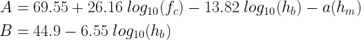
The generic closed form expression for path loss (PL) in dB scale, is given by
where, the Tx-Rx separation distance (d) is specified in kilometers (valid range 1 km to 20 Km). The factors A,B,C depend on the frequency of transmission, antenna heights and the type of environment, as given next.
● fc= frequency of transmission in MHz, valid range – 150 MHz to 1500 MHz ● hb= effective height of transmitting base station antenna in meters, valid range 30 m to 200 m ● hm=effective receiving mobile device antenna height in meters, valid range 1m to 10 m ● a(hm) = mobile antenna height correction factor that depends on the environment (refer table below) ● C = a factor used to correct the formulas for open rural and suburban areas (refer table below)
The function to simulate Hata-Okumura model is given in the book – Wireless Communication Systems using Matlab. The simulated path loss in three types of environments are plotted in Figure 1. The simulated results are obtained over a range of distances for the following parameter values fc=1500 MHz, hb=70 m and hm=1.5 m.
Rate this article: Note: There is a rating embedded within this post, please visit this post to rate it.
Key focus: Let’s learn how to simulate matched filter receiver with square root raised cosine (SRRC) filter, for a pulse amplitude modulation (PAM) system.
Simulation Model
A basic pulse amplitude modulation (PAM) system as DSP implementation, is shown in Figure 1 by adding an upsampler (), pulse shaping function () at the transmitter and a matched filter (), downsampler () combination at the receiver.
Figure 1: DSP implementation of a PAM modulation system with pulse shaping and matched filtering
In this model, a random stream of source bits is first segmented into -bit wide symbols that can take any value from the set . The simulation code directly starts by generating a random set of symbols, that goes into the modulation mapper. Pulse amplitude modulation (MPAM) mapping and de-mapping, described in sections 5.3.1 and 5.4.1, are considered here for simulation. An MPAM modulator maps the -bit information symbols to one of the distinct signaling levels. The MPAM modulated symbols are shown in Figure 2.
%Program: MPAM modulation
N = 10ˆ5; %Number of symbols to transmit
MOD_TYPE = 'PAM'; %modulation type
M = 4; %modulation level for the chosen modulation MOD_TYPE
d = ceil(M.*rand(1,N)); %random numbers from 1 to M for input to PAM
u = modulate(MOD_TYPE,M,d);%MPAM modulation
figure; stem(real(u)); %plot modulated symbols
Figure 2: M-PAM modulated Symbols
Each MPAM modulated symbol should last for some duration called symbol time, denoted as . Each modulated symbol will go through a discrete time pulse shaping filter whose impulse response is spaced sample, where denotes the sampling period. To do this, the incoming symbols from the modulation mapper need to be converted to discrete time impulse train by upsampling them by a factor (as per the upsampling equation given here ). The upsampler inserts zeros between each modulated symbols. In practice, is chosen as integral multiples of 4. The upsampler/oversampled output is shown in Figure 3.
%Program: Upsampling
L=4; %Oversampling factor (L samples per symbol period)
v=[u;zeros(L-1,length(u))];%insert L-1 zero between each symbols
%Convert to a single stream
v=v(:).';%now the output is at sampling rate
stem(real(v)); title('Oversampled symbols v(n)');
Figure 3: Modulated symbols upsampled by 4 (left) and the SRRC pulse shaping filter output (right)
In order to fill-in proper values in place of the inserted zeros, interpolation is performed by a pulse shaping filter by convolving the output of the upsampler and the pulse shaping function. The pulse shaping function needs to satisfy Nyquist criterion for zero ISI, otherwise, aliasing effect will wreak havoc. If the amplitude response of the channel is flat and if the noise is white, then the amplitude response of the pulse shaping function can be split equally between the transmitter and receiver. For this simulation the desired Nyquist pulse shape is a raised-cosine pulse shape and the task of raised-cosine filtering is equally split between the transmit and receive filters. This gives rise to square-root raised-cosine (SRRC) filters at the transmitter and receiver. This is a matched filter system, where the receive filter is matched with the transmit pulse shaping filter.
A matched filtering system is a theoretical framework and it is not a specific type of filter. It offers improved noise cancellation by improving the signal noise ratio at the output of the receive filter. The implementation starts with the design of an SRRC filter with roll-off factor . The SRRC filter length is influenced by the parameter – the span of the filter length in units of symbols and the oversampling factor .
Filters will not produce instantaneous output and they take sometime to produce the output. That is, the output of the filter is shifted in time with respect to the input. For symmetric FIR filters of length , the filter delay is . Apart from returning the SRRC pulse function, the filter design function given in this section returns the filter delay. Filter delays are useful in determining the appropriate sampling instances at the receiver. The modulated symbols at the transmitter are passed through the designed filter and the response of the filter is plotted in Figure 3 (right).
%Program: SRRC pulse shaping
%----Pulse shaping-----
beta = 0.3;% roll-off factor for Tx SRRC filter
Nsym=8;%SRRC filter span in symbol durations
L=4; %Oversampling factor (L samples per symbol period)
[p,t,filtDelay] = srrcFunction(beta,L,Nsym);%design filter
s=conv(v,p,'full');%Convolve modulated syms with p[n] filter
figure; plot(real(s),'r'); title('Pulse shaped symbols s(n)');
Figure 4: Received signal with AWGN noise (left) and the output of the matched filter (right)
The pulse shaped signal samples are sent through an AWGN channel, where the transmitted samples are added with noise samples that are generated according to the required (refer AWGN noise model given in this post). The received signal that is corrupted with AWGN noise is shown in Figure 4 (left).
%Program: Adding AWGN noise for given SNR value
EbN0dB = 10; %EbN0 in dB for AWGN channel
snr = 10*log10(log2(M))+EbN0dB; %Converting given Eb/N0 dB to SNR
%log2(M) gives the number of bits in each modulated symbol
r = add_awgn_noise(s,snr,L); %AWGN , add noise for given SNR, r=s+w
%L is the oversampling factor used in simulation
figure; plot(real(r),'r');title('Received signal r(n)');
For the receiver system, we assume that the ADC in the receiver produces an integer number of samples per symbol (i.e, is an integer). In practice, this is not always the case and thus a resampling filter is often included in real world designs. In the discrete time model, the received samples are passed through a matched filter, whose impulse response is matched to the impulse response of the pulse shaping filter as . Since the SRRC pulse is symmetric, we will be using the same SRRC pulse shaping function for the matched filter. The received samples are convolved with the matched filter and the output of the matched filter is shown in Figure 4 (right).
Next, we assume that the receiver has perfect knowledge of symbol timing instants and therefore, we will not be implementing a symbol timing synchronization subsystem in the receiver. At the receiver, the matched filter symbols are first passed through a downsampler that samples the filter output at correct timing instances.
The sampling instances are influenced by the delay of the FIR filters (SRRC filters in Tx and Rx). For symmetric FIR filters of length , the filter delay is . Since the communication link contains two filters, the total filter delay is . Therefore, the first valid sample occurs at position in the matched filter’s output vector ( is added due to the fact that Matlab array indices starts from 1). The downsampler that follows, starts to sample the signal from this position and returns every symbol. The downsampled output, shown in Figure 5, is then passed through a demodulator that decides on the symbols using an optimum detection technique and remaps them back to the intended message symbols.
Figure 5: Downsampling – output of symbol rate sampler
%Program: Symbol rate sampler and demodulation
%------Symbol rate Sampler-----
uCap = vCap(2*filtDelay+1:L:end-(2*filtDelay))/L;
%downsample by L from 2*filtdelay+1 position result by normalized L,
%as the matched filter result is scaled by L
figure; stem(real(uCap)); hold on;
title('After symbol rate sampler $\hat{u}$(n)',...
'Interpreter','Latex');
dCap = demodulate(MOD_TYPE,M,uCap); %demodulation
Rate this article: Note: There is a rating embedded within this post, please visit this post to rate it.
Intersymbol interference (ISI) is a common problem in telecommunication systems, such as terrestrial television broadcasting, digital data communication systems, and cellular mobile communication systems. Dispersive effects in high-speed data transmission and multipath fading are the main reasons for ISI. To maximize the capacity, the transmission bandwidth must be extended to the entire usable bandwidth of the channel and that also leads to ISI.
To mitigate the effect of ISI, equalization techniques can be applied at the receiver side. Under the assumption of correct decisions, a zero-forcing decision feedback equalization (ZF-DFE) completely removes the ISI and leaves the white noise uncolored. It was also shown that ZF-DFE in combination with powerful coding techniques, allows transmission to approach the channel capacity [1]. DFE is adaptive and works well in the presence of spectral nulls and hence suitable for various PR channels that has spectral nulls. However, DFE suffers from error propagation and is not flexible enough to incorporate itself with powerful channel coding techniques such as trellis-coded modulation (TCM) and low-density parity codes (LDPC).
These problems can be practically mitigated by employing precodingtechniques at the transmitter side. Precoding eliminates error propagation effects at the source if the channel state information is known precisely at the transmitter. Additionally, precoding at transmitter allows coding techniques to be incorporated in the same way as for channels without ISI. In this text, a partial response (PR) signaling system is taken as an example to demonstrate the concept of precoding.
Precoding system using filters
In a PR signaling scheme, a filter is used at the transmitter to introduce a controlled amount of ISI into the signal. The introduced ISI can be compensated for, at the receiver by employing an inverse filter . In the case of PR1 signaling, the filters would be
Generally, the filter is chosen to be of FIR type and therefore its inverse at the receiver will be of IIR type. If the received signal is affected by noise, the usage of IIR filter at the receiver is prone to error propagation. Therefore, instead of compensating for the ISI at the receiver, a precoder can be implemented at the transmitter as shown in Figure 1.
Figure 1: A pre-equalization system incorporating a modulo-M precoder
Since the precoder is of IIR type, the output can become unbounded. For example, let’s filter a binary data sequence through the precoder used for PR1 signaling scheme.
The result indicates that the output becomes unbounded and some additional measure has to be taken to limit the output. Assuming M-ary signaling schemes like MPAM is used for transmission, the unbounded output of the precoder can be bounded by incorporating modulo-M operation.
Rate this article: Note: There is a rating embedded within this post, please visit this post to rate it.
Reference
[1] R. Price, Nonlinear Feedback Equalized PAM versus Capacity for Noisy Filter Channels, in Proceedings of the Int. Conference on Comm. (ICC ’72), 1972, pp. 22.12-22.17
Impulse response and frequency response of PR signaling schemes
Consider a minimum bandwidth system in which the filter is represented as a cascaded combination of a partial response filter and a minimum bandwidth filter . Since is a brick-wall filter, the frequency response of the whole system is equivalent to frequency response of the FIR filter , whose transfer function, for various partial response schemes, was listed in Table 1 in the previous post (shown below).
Table 1: Partial response signaling schemes
The hand-crafted Matlab function (given in the book) generates the overall partial response signal for the given transfer function . The function records the impulse response of the filter by sending an impulse through it. These samples are computed at each symbol sampling instants. In order to visualize the pulse shaping functions and to compute the frequency response, the impulse response of are oversampled by a factor . This converts the samples from symbol rate domain to sampling rate domain. The oversampled impulse response of filter is convolved with a sinc filter that satisfies the Nyquist first criterion. This results in the overall response of the equivalent filter (refer Figure 2 in the previous post).
The Matlab code to simulate both the impulse response and the frequency response of various PR signaling schemes, is given next (refer book for the Matlab code). The simulated results are plotted in the following Figure.
Consider the generic baseband communication system model and its equivalent representation, shown in Figure 1, where the various blocks in the system are represented as filters. To have no ISI at the symbol sampling instants, the equivalent filter should satisfy Nyquist’s first criterion.
Figure 1: A generic communication system model and its equivalent representation
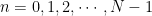
If the system is ideal and noiseless, it can be characterized by samples of the desired impulse response . Let’s represent all the non-zero sample values of the desired impulse response, taken at symbol sampling spacing , as , for .
The partial response signaling model, illustrated in Figure 2, is expressed as a cascaded combination of a tapped delay line filter with tap coefficients set to and a filter with frequency response . The filter forces the desired sample values. On the other hand, the filter bandlimits the system response and at the same time it preserves the sample values from the filter . The choice of filter coefficients for the filter and the different choices for for satisfying Nyquist first criterion, result in different impulse response , but renders identical sample values in Figure 2[1].
Figure 2: A generic partial response (PR) signaling model
To have a system with minimum possible bandwidth, the filter is chosen as
The inverse Fourier transform of results in a sinc pulse. The corresponding overall impulse response of the system is given by
If the bandwidth can be relaxed, other ISI free pulse-shapers like raised cosine can be considered for the filter.
Given the nature of real world channels, it is not always desirable to satisfy Nyquist’s first criterion. For example, the channel in magnetic recording, exhibits spectral null at certain frequencies and therefore it defines the channel’s upper frequency limit. In such cases, it is very difficult to satisfy Nyquist first criterion. An alternative viable solution is to allow a controlled amount of ISI between the adjacent samples at the output of the equivalent filter shown in Figure 2. This deliberate injection of controlled amount of ISI is called partial response (PR) signaling or correlative coding.
Partial Response Signaling Schemes
Several classes of PR signaling schemes and their corresponding transfer functions represented as (where is the delay operator) are shown in Table 1. The unit delay is equal to a delay of 1 symbol duration () in a continuous time system.
Eye diagram is a powerful tool to analyze the overall quality of a communication link. It reveals important characteristics of a communication link, that includes timing sensitivity, noise margin, inter-symbol interference (ISI) and zero-crossing jitter. It also shows the optimum sampling time for the receiver, which indicates when to sample the incoming signal for converting it to a symbol stream. It is more useful to plot the eye diagram at the receiver, where it gives visual cues for the engineers to check the signal integrity and to uncover problems in earlier stages of the design process.
Application of eye diagram
For each symbol received through a noisy channel, the receiver has to make the best estimate of what was transmitted. Eventually, this boils down to finding out the optimal decision time for each symbol (through timing recovery circuits) after the signal is processed through the equalizer and the matched filter.
In an eye diagram, each period of the waveform is repeated and overlaid on top of each other, forming an eye like pattern. It is usually visualized at the point just prior to the decisions. It reveals the ability of the receiver to distinguish between signal levels, in the presence of distortions like timing jitters (due to imperfect recovered clocks), noise level in the received signal prior to decision point, etc..,
An ideal eye diagram will show a wider eye that has a lot of margin in both horizontal and vertical direction that allows for lowest possible error rate in the receiver decisions. Figure 1, depicts the eye diagram for 2-PAM modulated square-root raised cosine (β=1) pulse shaped symbols sent through an AWGN channel having EbN0=50 dB (almost no noise condition).
Figure 1: Ideal eye diagram shown for two symbol durations for 2-PAM modulation shaped using square root raised cosine filters.
A narrower eye implies increased sensitivity to noise, since presence of more noise would cause erroneous symbol decisions. In essence, erroneous symbol decisions could be caused by timing jitters (measured in the horizontal direction) or the amplitude variation (measured in the vertical direction) or intersymbol interference (which affects the signal in both directions). Figure 2, depicts the eye diagram for 2-PAM modulated symbols sent through an AWGN channel having EbN0=20 dB (signal to noise ratio).
Figure 2: Eye diagram shown for 2-PAM modulated pulse shaped symbols corrupted with AWGN noise (EbN0=20 dB)
Construction of eye diagrams from signals represented in computer memory.
To construct an eye diagram, the signal is divided into equal sections. The number of samples in each section should be proportional to , where is the symbol period (which is related to the oversampling factor by equation (1).
The factor denotes the oversampling factor or upsampling ratio which is given as the ratio of symbol period () and the sampling period () or equivalently, the ratio of sampling rate and the symbol rate
When all such sections are plotted in an overlapping manner, it produces the eye diagram. This is implemented in the following Matlab function. The sample usage of the function is given in the next section of this chapter and the sample outputs are available in the following Figure.
function [eyeVals]=plotEyeDiagram(x,L,nSamples,offset,nTraces)
%Function to plot eye diagram
%x - input vector representing the signal
%L - oversampling factor (for calculating x-axis in plot)
%nSamples - number of samples per trace - preferably set to integral
% multiple of oversampling factor L(number of bits per symbol)
%offset - initial offset in the data from where to begin plotting
%nTraces - number of traces to plot
%If the signal processing toolbox is not available, put M=1
% and convert the line that says y=interp(x,M) to y=x

.....
Refer the book Wireless Communication systems using Matlab
.....
end
Rate this article: Note: There is a rating embedded within this post, please visit this post to rate it.
Let’s learn the equations and the filter model for simulating square root raised cosine (SRRC) pulse shaping. Before proceeding, I urge you to read about basics of pulse shaping in this article.
Figure 1: Combined response of two SRRC filters and frequency domain view of a single SRRC pulse
Raised-cosine pulse shaping filter is generally employed at the transmitter. Let be the raised cosine filter’s frequency response. Assume that the channel’s amplitude response is flat, i.e, and the channel noise is white. Then, the combined response of the transmit filter and receiver filter in frequency domain is given as
If the receive filter is matched with the transmit filter, we have
Thus, the transmit and the receive filter take the form
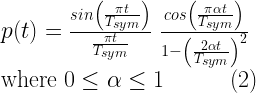
with , where is a nominal delay that is required to ensure the practical realizability of the filters. In time domain, a matched filter at the receiver is the mirrored copy of the impulse response of the transmit pulse shaping filter and is delayed by some time . Thus the task of raised cosine filtering is equally split between the transmit and receive filters. This gives rise to square-root raised-cosine (SRRC) filters at the transmitter and receiver, whose equivalent impulse response is described as follows.
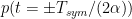
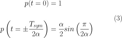
The roll-of factor for the SRRC is denoted as to distinguish it from that of the RC filter. A simple evaluation of the equation (4) produces singularities (undefined points) at and . The value of the square root raised cosine pulse at these singularities can be obtained by applying L’Hostipital’s rule [1] and the values are
A function for generating SRRC pulse shape is given next. It is followed by a test code that plots the combined impulse response of transmit-receive SRRC filter combination and also plots the frequency domain view of a single SRRC pulse as shown in Figure 1
The combined impulse response matters, as we can identify that the combined response hits zero at symbol sampling instants. This indicates that the job of ISI cancellation is split between transmitter and receiver filters. Note that the combined impulse response of two SRRC filters is same as the impulse response of the RC filter.
Program 2: test_SRRCPulse.m: Square-root raised-cosine pulse characteristics
Tsym=1; %Symbol duration in seconds
L=10; % oversampling rate, each symbol contains L samples
Nsym = 80; %filter span in symbol durations
betas=[0 0.22 0.5 1];%root raised-cosine roll-off factors
Fs=L/Tsym;%sampling frequency
lineColors=['b','r','g','k','c']; i=1;legendString=cell(1,4);
for beta=betas %loop for various alpha values
	[srrcPulseAtTx,t]=srrcFunction(beta,L,Nsym); %SRRC Filter at Tx
	srrcPulseAtRx = srrcPulseAtTx;%Using the same filter at Rx
	%Combined response matters as it hits 0 at desired sampling instants
	combinedResponse = conv(srrcPulseAtTx,srrcPulseAtRx,'same');

	subplot(1,2,1); t=Tsym*t; %translate time base & normalize reponse
	plot(t,combinedResponse/max(combinedResponse),lineColors(i));
	hold on;

	%See Chapter 1 for the function 'freqDomainView'
	[vals,F]=freqDomainView(srrcPulseAtTx,Fs,'double');
	subplot(1,2,2);
	plot(F,abs(vals)/abs(vals(length(vals)/2+1)),lineColors(i));
	hold on;legendString{i}=strcat('\beta =',num2str(beta) );i=i+1;
end
subplot(1,2,1);
title('Combined response of SRRC filters'); legend(legendString);
subplot(1,2,2);
title('Frequency response (at Tx/Rx only)');legend(legendString);
As mentioned earlier, the shortcomings of the sinc pulse can be addressed by making the transition band in the frequency domain less abrupt. The raised-cosine(RC) pulse comes with an adjustable transition band roll-off parameter , using which the transition band’s rate of decay can be controlled. The RC pulse shaping function is expressed in frequency domain as
Correspondingly, in time domain, the impulse response is given by
A simple evaluation of the equation (2) produces singularities (undefined points) at and . The value of the raised-cosine pulse at these singularities can be obtained by applying L’Hospital’s rule [1] and the values are
Figure 1: Raised-cosine pulse and its manifestation in frequency domain
The following Matlab codes generate a raised cosine pulse for the given symbol duration and plot the time-domain view and the frequency response (shown in Figure 1). The RC pulse falls off at the rate of as , which is a significant improvement when compared to the decay rate of sinc pulse which is . It satisfies Nyquist criterion for zero ISI – the pulse hits zero crossings at desired sampling instants. By controlling , the transition band roll-off in the frequency domain can be made gradual.
Program 2: test_RCPulse.m: Raised-cosine pulses and their manifestation in frequency domain
Tsym=1; %Symbol duration in seconds
L=10; % oversampling rate, each symbol contains L samples
Nsym = 80; %filter span in symbol durations
alphas=[0 0.3 0.5 1];%RC roll-off factors - valid range 0 to 1
Fs=L/Tsym;%sampling frequency
lineColors=['b','r','g','k','c']; i=1;legendString=cell(1,4);

for alpha=alphas %loop for various alpha values
	[rcPulse,t]=raisedCosineFunction(alpha,L,Nsym); %RC Pulse

	subplot(1,2,1); t=Tsym*t; %translate time base for given duration
	plot(t,rcPulse,lineColors(i));hold on; %plot time domain view
	[vals,f]=freqDomainView(rcPulse,Fs,'double');%See Chapter 1

	subplot(1,2,2);
	plot(f,abs(vals)/abs(vals(length(vals)/2+1)),lineColors(i));
	hold on;legendString{i}=strcat('\alpha =',num2str(alpha) );i=i+1;
end
subplot(1,2,1);title('Raised Cosine pulse'); legend(legendString);
subplot(1,2,2);title('Frequency response');legend(legendString);
References
[1] Clay S. Turner, Raised cosine and root raised cosine formulae, Wireless Systems Engineering, Inc, May 29, 2007.
Rate this post: Note: There is a rating embedded within this post, please visit this post to rate it.
Key focus: Sinc pulse shaping of transmitted bits, offers minimum bandwidth and avoids intersymbol interference. Discuss its practical considerations & simulation.
Sinc pulse shaping
As suggested in the earlier post, the pulse shape that avoids ISI with the least amount of bandwidth is a sinc pulse of bandwidth . Here, is the baud rate of the system also called symbol rate. A sinc pulse described as time and frequency domain dual is given below
Following Matlab codes generate a sinc pulse with and plot the time-domain/frequency-domain response (Figure 1). From the time-domain plot, the value of the sinc pulse hits zero at integral multiple sampling instants seconds except at where it peaks to the maximum value. Thus the sinc pulse satisfies the Nyquist criterion for zero ISI.
Program 2: Sinc pulse and its manifestation in frequency domain
Tsym=1; %Symbol duration
L=16; %oversampling rate, each symbol contains L samples
Nsym = 80; %filter span in symbol duration
Fs=L/Tsym; %sampling frequency
[p,t]=sincFunction(L,Nsym); %Sinc Pulse
subplot(1,2,1); t=t*Tsym; plot(t,p); title('Sinc pulse');
[fftVals,freqVals]=freqDomainView(p,Fs,'double'); %See Chapter 1
subplot(1,2,2);
plot(freqVals,abs(fftVals)/abs(fftVals(length(fftVals)/2+1)));
Figure 1: Sinc pulse and its manifestation in frequency domain
The main drawback of the sinc pulse is that it decays too slowly at the rate of as . This implies that the samples that are far apart can cause intersymbol interference in the event of modest clock synchronization errors. A sinc pulse is of infinite duration and for practical implementations, it has to be truncated to finite length for some integer . This leads to problems in frequency domain as explained next.
Figure 2 shows the one-sided frequency response of the sinc pulse that is truncated to various lengths. It is evident that the truncation of sinc pulse in time domain to leads to sidelobes in the frequency domain and the sidelobes become wider for decreasing values of . This effect is closely related to Gibbs phenomenon – the ringing artifact due to approximation of discontinuities by spectral methods. As a result, no matter how large the value of is chosen, the first sidelobe is always only down from the main lobe. Also, the sinc pulse is very sensitive to the timing jitters at the receiver. These problems can be addressed when the transition band in the frequency domain is made less abrupt.
Rate this article: Note: There is a rating embedded within this post, please visit this post to rate it.
This website uses cookies to improve your experience while you navigate through the website. Out of these, the cookies that are categorized as necessary are stored on your browser as they are essential for the working of basic functionalities of the website. We also use third-party cookies that help us analyze and understand how you use this website. These cookies will be stored in your browser only with your consent. You also have the option to opt-out of these cookies. But opting out of some of these cookies may affect your browsing experience.
Necessary cookies are absolutely essential for the website to function properly. These cookies ensure basic functionalities and security features of the website, anonymously.
Cookie
Duration
Description
cookielawinfo-checbox-analytics
11 months
This cookie is set by GDPR Cookie Consent plugin. The cookie is used to store the user consent for the cookies in the category "Analytics".
cookielawinfo-checbox-analytics
11 months
This cookie is set by GDPR Cookie Consent plugin. The cookie is used to store the user consent for the cookies in the category "Analytics".
cookielawinfo-checbox-functional
11 months
The cookie is set by GDPR cookie consent to record the user consent for the cookies in the category "Functional".
cookielawinfo-checbox-functional
11 months
The cookie is set by GDPR cookie consent to record the user consent for the cookies in the category "Functional".
cookielawinfo-checbox-others
11 months
This cookie is set by GDPR Cookie Consent plugin. The cookie is used to store the user consent for the cookies in the category "Other.
cookielawinfo-checbox-others
11 months
This cookie is set by GDPR Cookie Consent plugin. The cookie is used to store the user consent for the cookies in the category "Other.
cookielawinfo-checkbox-necessary
11 months
This cookie is set by GDPR Cookie Consent plugin. The cookies is used to store the user consent for the cookies in the category "Necessary".
cookielawinfo-checkbox-performance
11 months
This cookie is set by GDPR Cookie Consent plugin. The cookie is used to store the user consent for the cookies in the category "Performance".
viewed_cookie_policy
11 months
The cookie is set by the GDPR Cookie Consent plugin and is used to store whether or not user has consented to the use of cookies. It does not store any personal data.
Functional cookies help to perform certain functionalities like sharing the content of the website on social media platforms, collect feedbacks, and other third-party features.
Performance cookies are used to understand and analyze the key performance indexes of the website which helps in delivering a better user experience for the visitors.
Analytical cookies are used to understand how visitors interact with the website. These cookies help provide information on metrics the number of visitors, bounce rate, traffic source, etc.


![p[n]](https://s0.wp.com/latex.php?latex=p%5Bn%5D&bg=ffffff&fg=000&s=0&c=20201002)

![g[n]](https://s0.wp.com/latex.php?latex=g%5Bn%5D&bg=ffffff&fg=000&s=0&c=20201002)


![g[n]=p[-n]](https://s0.wp.com/latex.php?latex=g%5Bn%5D%3Dp%5B-n%5D&bg=ffffff&fg=000&s=0&c=20201002)


![[Q(z)]^{-1}](https://s0.wp.com/latex.php?latex=%5BQ%28z%29%5D%5E%7B-1%7D&bg=ffffff&fg=000&s=0&c=20201002)


![d_n=\left[1,0,1,0,1,0,1,0,1,0\right]](https://s0.wp.com/latex.php?latex=d_n%3D%5Cleft%5B1%2C0%2C1%2C0%2C1%2C0%2C1%2C0%2C1%2C0%5Cright%5D&bg=ffffff&fg=000&s=0&c=20201002)

![[Q(z)]^{-1}=(1+z^{-1})^{-1}](https://s0.wp.com/latex.php?latex=%5BQ%28z%29%5D%5E%7B-1%7D%3D%281%2Bz%5E%7B-1%7D%29%5E%7B-1%7D&bg=ffffff&fg=000&s=0&c=20201002)