Young’s fading channel model is a mathematical model used to describe the behavior of a wireless communication channel. It is a type of frequency selective fading channel model that is commonly used to simulate the effects of multipath interference on wireless signals.
The model is based on the assumption that the transmitted signal reaches the receiver through multiple paths, each with a different attenuation and phase shift. The attenuation and phase shift of each path are modeled as independent random variables with specific probability distributions.
The model uses the sum of these attenuated and phase-shifted paths to simulate the received signal. The resulting signal experiences fading due to the constructive and destructive interference of the individual paths.
Young’s fading channel model is useful for simulating the performance of wireless communication systems in a multipath environment. It can help researchers and engineers evaluate the performance of different modulation and coding schemes and develop techniques to mitigate the effects of fading.
Young’s model
In the previous article, the characteristics and types of fading was discussed. Rayleigh Fading channel with Doppler shift is considered in this article.
Consider a channel affected by both Rayleigh Fading phenomena and Doppler Shift. Rayleigh Fading is caused due to multipath reflections of the received signal before it reaches the receiver and the Doppler Shift is caused due to the difference in the relative velocity/motion between the transmitter and the receiver. This scenario is encountered in day to day mobile communications.
A number of simulation algorithms are proposed for generation of correlated Rayleigh random variables. David J.Young and Norman C Beaulieu proposed a method in their paper titled “The Generation of Correlated Rayleigh Random Variates by Inverse Discrete Fourier Transform”[1] based on the inverse discrete Fourier transform (IDFT). It is a modification of the Smith’s algorithm which is normally used for Rayleigh fading simulation. This method requires exactly one-half the number of IDFT operations and roughly two-thirds the computer memory of the original method – as the authors of the paper claims.
Rayleigh Fading can be simulated by adding two Gaussian Random variables as mentioned in my previous post. The effect of Doppler shift is incorporated by modeling the Doppler effect as a frequency domain filter.
The model proposed by Young et.al is shown below.
Rayleigh Fading – Young’s model
The Fading effect + Doppler Shift is simulated by multiplying the Gaussian Random variables and the Doppler Shift’s Frequency domain representation. Then IDFT is performed to bring them into time domain representation. The Doppler Filter used to represent the Doppler Shift effect is derived in Young’s paper.
Keyfocus: Fading channel models for simulation. Learn how fading channels can be modeled as FIR filters for simplified modulation & detection. Rayleigh/Rician fading.
Introduction
A fading channel is a wireless communication channel in which the quality of the signal fluctuates over time due to changes in the transmission environment. These changes can be caused by different factors such as distance, obstacles, and interference, resulting in attenuation and phase shifting. The signal fluctuations can cause errors or loss of information during transmission.
Fading channels are categorized into slow fading and fast fading depending on the rate of channel variation. Slow fading occurs over long periods, while fast fading happens rapidly over short periods, typically due to multipath interference.
To overcome the negative effects of fading, various techniques are used, including diversity techniques, equalization, and channel coding.
Fading channel in frequency domain
With respect to the frequency domain characteristics, the fading channels can be classified into frequency selective and frequency-flat fading.
A frequency flat fading channel is a wireless communication channel where the attenuation and phase shift of the signal are constant across the entire frequency band. This means that the signal experiences the same amount of fading at all frequencies, and there is no frequency-dependent distortion of the signal.
In contrast, a frequency selective fading channel is a wireless communication channel where the attenuation and phase shift of the signal vary with frequency. This means that the signal experiences different levels of fading at different frequencies, resulting in a frequency-dependent distortion of the signal.
Frequency selective fading can occur due to various factors such as multipath interference and the presence of objects that scatter or absorb certain frequencies more than others. To mitigate the effects of frequency selective fading, various techniques can be used, such as equalization and frequency hopping.
The channel fading can be modeled with different statistics like Rayleigh, Rician, Nakagami fading. The fading channel models, in this section, are utilized for obtaining the simulated performance of various modulations over Rayleigh flat fading and Rician flat fading channels. Modeling of frequency selective fading channel is discussed in this article.
Linear time invariant channel model and FIR filters
The most significant feature of a real world channel is that the channel does not immediately respond to the input. Physically, this indicates some sort of inertia built into the channel/medium, that takes some time to respond. As a consequence, it may introduce distortion effects like inter-symbol interference (ISI) at the channel output. Such effects are best studied with the linear time invariant (LTI) channel model, given in Figure 1.
Figure 1: Complex baseband equivalent LTI channel model
In this model, the channel response to any input depends only on the channel impulse response(CIR) function of the channel. The CIR is usually defined for finite length \(L\) as \(\mathbf{h}=[h_0,h_1,h_2, \cdots,h_{L-1}]\) where \(h_0\) is the CIR at symbol sampling instant \(0T_{sym}\) and \(h_{L-1}\) is the CIR at symbol sampling instant \((L-1)T_{sym}\). Such a channel can be modeled as a tapped delay line (TDL) filter, otherwise called finite impulse response (FIR) filter. Here, we only consider the CIR at symbol sampling instances. It is well known that the output of such a channel (\(\mathbf{r}\)) is given as the linear convolution of the input symbols (\(\mathbf{s}\)) and the CIR (\(\mathbf{h}\)) at symbol sampling instances. In addition, channel noise in the form of AWGN can also be included the model. Therefore, the resulting vector of from the entire channel model is given as
Simulation model for detection in flat fading channel
A flat-fading (also called as frequency-non-selective) channel is modeled with a single tap (\(L=1\)) FIR filter with the tap weights drawn from distributions like Rayleigh, Rician or Nakagami distributions. We will assume block fading, which implies that the fading process is approximately constant for a given transmission interval. For block fading, the random tap coefficient \(h=h[0]\) is a complex random variable (not random processes) and for each channel realization, a new set of complex random values are drawn from Rayleigh or Rician or Nakagami fading according to the type of fading desired.
Figure 2: LTI channel viewed as tapped delay line filter
Simulation models for modulation and detection over a fading channel is shown in Figure 2. For a flat fading channel, the output of the channel can be expressed simply as the product of time varying channel response and the input signal. Thus, equation (1) can be simplified (refer this article for derivation) as follows for the flat fading channel.
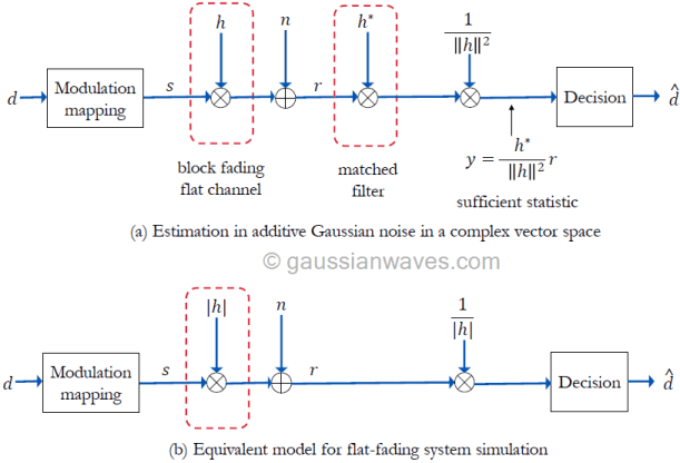
Since the channel and noise are modeled as a complex vectors, the detection of \(\mathbf{s}\) from the received signal is an estimation problem in the complex vector space.
Assuming perfect channel knowledge at the receiver and coherent detection, the receiver shown in Figure 3(a) performs matched filtering. The impulse response of the matched filter is matched to the impulse response of the flat-fading channel as \( h^{\ast}\). The output of the matched filter is scaled down by a factor of \(||h||^2\) which is the total-energy contained in the impulse response of the flat-fading channel. The resulting decision vector \(\mathbf{y}\) serves as the sufficient statistic for the estimation of \(\mathbf{s}\) from the received signal \(\mathbf{r}\) (refer equation A.77 in reference [1])
Since the absolute value \(|h|\) and the Eucliden norm \(||h||\) are related as \(|h|^2= \left\lVert h\right\rVert = hh^{\ast}\), the model can be simplified further as given in Figure 3(b).
To simulate flat fading, the values for the fading variable \(h\) are drawn from complex normal distribution
\[h= X + jY \quad\quad (4) \]
where, \(X,Y\) are statistically independent real valued normal random variables.
● If \(E[h]=0\), then \(|h|\) is Rayleigh distributed, resulting in a Rayleigh flat fading channel ● If \(E[h] \neq 0\), then \(|h|\) is Rician distributed, resulting in a Rician flat fading channel with the factor \(K=[E[h]]^2/\sigma^2_h\)
The central limit theorem (CLT) is a fundamental concept in statistics and probability theory that explains how the sum of independent and identically distributed random variables behaves. The theorem states that as the number of these variables increases, the distribution of their sum tends to become more like a normal distribution, even if the variables themselves are not normally distributed.
CLT states that the sum of independent and identically distributed (i.i.d)random variables (with finite mean and variance) approaches normal distribution as sample size \(N \rightarrow \infty\). In simpler terms, the theorem states that under certain general conditions, the sum of independent observations that follow same underlying distribution approximates to normal distribution. The approximation steadily improves as the number of observations increase. The underlying distribution of the independent observation can be anything – binomial, Poisson, exponential, Chi-Squared etc.
Why CLT ?
CLT is an important concept in statistics because it allows us to make inferences about a population based on a sample, even if we do not know the distribution of the population. It is used in many statistical techniques, such as hypothesis testing and confidence intervals.
Applications of CLT
Central limit theorem (CLT) is applied in a vast range of applications including (but not limited to) signal processing, channel modeling, random process, population statistics, engineering research, predicting the confidence intervals, hypothesis testing, etc. One such application in signal processing is – deriving the response of a cascaded series of low pass filters by applying the CLT. In the article titled ‘the central limit theorem and low-pass filters‘ the author has illustrated how the response of a cascaded series of low pass filters approaches Gaussian shape as the number of filters in the series increase [1].
In digital communication, the effect of noise on a communication channel is modeled as additive Gaussian white noise. This follows from the fact that the noise from many physical channels can be considered approximately Gaussian. For example, the random movement of electrons in the semiconductor devices gives rise to shot noise whose effect can be approximated to Gaussian distribution by applying central limit theorem.
Law of large numbers and CLT
there is a connection between the central limit theorem and the law of large numbers.
The law of large numbers is another important theorem in probability theory, which states that as the number of independent and identically distributed (iid) random variables increases, the average of those variables converges to the expected value of the distribution. In other words, as the sample size increases, the sample mean becomes more and more representative of the true population mean.
The central limit theorem, on the other hand, describes the distribution of the sum of iid random variables, and shows that as the sample size increases, the distribution of the sum approaches a normal distribution.
Both the law of large numbers and the CLT deal with the behavior of the sum or average of iid random variables as the sample size gets larger. The law of large numbers describes the behavior of the sample mean, while the CLT describes the behavior of the sum of the variables.
In essence, the law of large numbers is a precursor to the central limit theorem, as it establishes the fact that the sample mean becomes more and more representative of the true population mean as the sample size increases, and the central limit theorem shows that the distribution of the sum of iid random variables approaches a normal distribution as the sample size gets larger.
The following Python code illustrate how the theorem comes to play when the number of observations is increased for two separate experiments: rolling \(N\) unbiased dice and tossing \(N\) unbiased coins. The code generates \(N\) i.i.d discrete uniform random variables that generates uniform random numbers from the set \(\left\{1,k\right\}\). In the case of the dice rolling experiment, \(k\) is set to \(6\), thus simulating the random pick from the sample space \(S=\left\{1,2,3,4,5,6\right\}\) with equal probability. For the coin tossing experiment, \(k\) is set to \(2\), thus simulating the sample space of \(S=\left\{1,2\right\}\) representing head or tail events with equal probability. Rest of the code is self explanatory.
Python code
#---------Central limit theorem - Author: Mathuranathan #gaussianwaves.com -----------------------
#
import numpy as np
import matplotlib.pyplot as plt
#%matplotlib inline

numIterations = np.asarray([1,2,5,10,50,100]); #number of i.i.d RVs
experiment = 'dice' #valid values: 'dice', 'coins'
maxNumForExperiment = {'dice':6,'coins':2} #max numbers represented on dice or coins
nSamp=100000

k = maxNumForExperiment[experiment]

fig, fig_axes = plt.subplots(ncols=3, nrows=2, constrained_layout=True)

for i,N in enumerate(numIterations):
    y = np.random.randint(low=1,high=k+1,size=(N,nSamp)).sum(axis=0)
    row = i//3;col=i%3;
    bins=np.arange(start=min(y),stop=max(y)+2,step=1)
    fig_axes[row,col].hist(y,bins=bins,density=True)
    fig_axes[row,col].set_title('N={} {}'.format(N,experiment))
plt.show()
Figure 1: Demonstrating central limit theorem using N numbers of dice
Figure 2: Demonstrating central limit theorem using N numbers of coins
Its been too long since I posted. For a kick start , i am continuing the theory on RS coding. Here is a simple Matlab code (which can be found in Matlab Help, posted here with a little bit detailed explanation) for better understanding of RS code
%Matlab Code for RS coding and decoding
n=7; k=3; % Codeword and message word lengths m=3; % Number of bits per symbol msg = gf([5 2 3; 0 1 7;3 6 1],m) % Two k-symbol message words % message vector is defined over a Galois field where the number must %range from 0 to 2^m-1
codedMessage = rsenc(msg,n,k) % Two n-symbol codewords
dmin=n-k+1 % display dmin t=(dmin-1)/2 % diplay error correcting capability of the code
% Generate noise – Add 2 contiguous symbol errors with first word; % 2 discontiguous symbol errors with second word and 3 distributed symbol % errors to last word noise=gf([0 0 0 2 3 0 0 ;6 0 1 0 0 0 0 ;5 0 6 0 0 4 0],m)
received = noise+codedMessage
%dec contains the decoded message and cnumerr contains the number of %symbols errors corrected for each row. Also if cnumerr(i) = -1 it indicates %that the ith row contains unrecoverable error [dec,cnumerr] = rsdec(received,n,k) % print the original message for comparison msg
% Given below is the output of the program. Only decoded message, cnumerr and original % message are given here (with comments inline)
% The default primitive polynomial over which the GF is defined is D^3+D+1 ( which is 1011 -> 11 in decimal).
dec = GF(2^3) array. Primitive polynomial = D^3+D+1 (11 decimal)
Array elements =
5 2 3 0 1 7 6 6 7
cnumerr =
2 2 -1 ->>> Error in last row -> this error is due to the fact that we have added 3 distributed errors with the last row where as the RS code can correct only 2 errors. Compare the decoded message with original message given below for confirmation
% Original message printed for comparison msg = GF(2^3) array. Primitive polynomial = D^3+D+1 (11 decimal)
Array elements =
5 2 3 0 1 7 3 6 1
Reference : [1] Mathematics behind RS codes – Bernard Sklar – Click Here
Keywords: Hamming code, error-correction code, digital communication, data storage, reliable transmission, computer memory systems, satellite communication systems, single-bit error, two-bit errors.
What is a Hamming Code
Hamming codes are a class of error-correcting codes that are commonly employed in digital communication and data storage systems to detect and correct errors that may occur during transmission or storage. They were created by Richard Hamming in the 1950s and bear his name.
The central concept of Hamming codes is to introduce additional (redundant) bits to a message in order to enable the identification and correction of errors. By appending parity bits to the original message, Hamming codes can identify and correct single-bit errors.
One notable characteristic of these codes is their ability to correct any single-bit error and detect any two-bit error, which has contributed to their widespread usage in computer memory systems, satellite communication systems, and other domains where reliable data transmission is crucial.
Technical details of Hamming code
Linear binary Hamming code falls under the category of linear block codes that can correct single bit errors. For every integer p ≥ 3 (the number of parity bits), there is a (2p-1, 2p-p-1) Hamming code. Here, 2p-1 is the number of symbols in the encoded codeword and 2p-p-1 is the number of information symbols the encoder can accept at a time. All such Hamming codes have a minimum Hamming distance dmin=3 and thus they can correct any single bit error and detect any two bit errors in the received vector. The characteristics of a generic (n,k) Hamming code is given below.
\[\begin{aligned} \text{Codeword length:} \quad && n &= 2^p-1 \\ \text{Number of information symbols:} \quad && k &= 2^p-p-1 \\ \text{Number of parity symbols:} \quad && n-k &= p \\ \text{Minimum distance:} \quad && d_{min} &= 3 \\ \text{Error correcting capability:} \quad && t &=1 \end{aligned}\]
With the simplest configuration: p=3, we get the most basic (7, 4) binary Hamming code. The (7,4) binary Hamming block encoder accepts blocks of 4-bit of information, adds 3 parity bits to each such block and produces 7-bits wide Hamming coded blocks.
Systematic & Non-systematic encoding
Block codes like Hamming codes are also classified into two categories that differ in terms of structure of the encoder output:
● Systematic encoding ● Non-systematic encoding
In systematic encoding, just by seeing the output of an encoder, we can separate the data and the redundant bits (also called parity bits). In the non-systematic encoding, the redundant bits and data bits are interspersed.
Figure 1: Systematic encoding and non-systematic encoding
Constructing (7,4) Hamming code
Hamming codes can be implemented in systematic or non-systematic form. A systematic linear block code can be converted to non-systematic form by elementary matrix transformations. A non-systematic Hamming code is described next.
Let a codeword belonging to (7, 4) Hamming code be represented by [D7,D6,D5,P4,D3,P2,P1], where D represents information bits and P represents parity bits at respective bit positions. The subscripts indicate the left to right position taken by the data and the parity bits. We note that the parity bits are located at position that are powers of two (bit positions 1,2,4).
Now, represent the bit positions in binary.
Seeing from left to right, the first parity bit (P1) covers the bits at positions whose binary representation has 1 at the least significant bit. We find that P1 covers the following bit positions
Similarly, the second parity bit (P2) covers the bits at positions whose binary representation has 1 at the second least significant bit. Hence, P2covers the following bit positions.
Finally, the third parity bit (P4) covers the bits at positions whose binary representation has 1 at the most significant bit. Hence, P4 covers the following bit positions
If we follow even parity scheme for parity bits, the number of 1’s covered by the parity bits must add up to an even number. Which implies that the XOR of bits covered by the parity (including the parity bits) must result in 0. Therefore, the following equations hold.
Following table illustrates the concept of constructing the Hamming code as described by R.W Hamming in his groundbreaking paper [1].
Table 1: Construction of (7,4) binary Hamming code
We note that the parity bits and data columns are interspersed. This is an example of non-systematic Hamming code structure. We can continue our work on the table above as it is. Or, we can also re-arrange the entries of that table using elemental transformations, such that a systematic Hamming code is rendered.
Figure 2: Re-arranging Hamming code using transformation (non-systematic to systematic code)
After the re-arrangement of columns, we see that the parity columns are nicely clubbed together at the end. We can also drop the subscripts given to the parity/data locations and re-index them according to our convenience. This gives the following structure to the (7,4) Hamming code.
Figure 3: Example for Systematic Hamming code
We will use the above systematic structure in the following discussion.
Encoding process
Given the structure in Figure 3, the parity bits are calculated from the following linearly independent equations using modulo-2 additions.
Figure 4: Computing the parity bits for (7,4) Hamming code
At the transmitter side, a Hamming encoder implements a generator matrix – . It is easier to construct the generator matrix from the linear equations listed in equation above. The linear equations show that the information bit D1 influences the calculation of parities at P1 and P3 . Similarly, the information bit D2 influences P1 and P2, D3 influences P1, P2 & P3 and D4 influences P2 & P3.
Represented as matrix operations, the encoder accepts 4 bit message block \(\mathbf{m}\), multiplies it with the generator matrix \(\mathbf{G}\) and generates 7 bit codewords \(\mathbf{c}\). Note that all the operations (addition, multiplication etc.,) are in modulo-2 domain.
\[\mathbf{c}= \mathbf{m} \mathbf{G} \]
Given a generator matrix, the Matlab code snippet for generating a codebook containing all possible codewords (\(\mathbf{c} \in \mathbf{C}\)) is given below. The resulting codebook \(\mathbf{C}\) can be used as a Look-Up-Table (LUT) when implementing the encoder. This implementation will avoid repeated multiplication of the input blocks and the generator matrix. The list of all possible codewords for the generator matrix (\(\mathbf{G}\)) given above are listed in table 2.
Table 2: All possible codewords for (7,4) Hamming code
Program: Generating all possible codewords from Generator matrix
%program to generate all possible codewords for (7,4) Hamming code
G=[ 1 0 0 0 1 0 1;
0 1 0 0 1 1 0;
0 0 1 0 1 1 1;
0 0 0 1 0 1 1];%generator matrix - (7,4) Hamming code
m=de2bi(0:1:15,'left-msb');%list of all numbers from 0 to 2ˆk
codebook=mod(m*G,2) %list of all possible codewords
Decoding process – Syndrome decoding
The three check equations for the given generator matrix (\(\mathbf{G}\)) for the sample (7,4) Hamming code, can be expressed collectively as a parity check matrix – \(\mathbf{H}\). Parity check matrix finds its usefulness in the receiver side for error-detection and error-correction.
According to parity-check theorem, for every generator matrix G, there exists a parity-check matrix H, that spans the null-space of G. Therefore, if c is a valid codeword, then it will be orthogonal to each row of H.
\[\mathbf{c} \mathbf{H}^T = 0 \]
Therefore, if \(\mathbf{H}\) is the parity-check matrix for a codebook \(\mathbf{C}\), then a vector \(\mathbf{c}\) in the received code space is a valid codeword if and only if it satisfies \(\mathbf{c} \mathbf{H}^T=0\).
Consider a vector of received word \(\mathbf{r}=\mathbf{c}+\mathbf{e}\), where \(\mathbf{c}\) is a valid codeword transmitted and \(\mathbf{e}\) is the error introduced by the channel. The matrix product \(\mathbf{r}\mathbf{H}^T\) is defined as the syndrome for the received vector \(\mathbf{r}\), which can be thought of as a linear transformation whose null space is \(\mathbf{C}\) [2].
Thus, the syndrome is independent of the transmitted codeword \(\mathbf{c}\) and is solely a function of the error pattern \(\mathbf{e}\). It can be determined that if two error vectors \(\mathbf{e}\) and \(\mathbf{e}’\) have the same syndrome, then the error vectors must differ by a nonzero codeword.
It follows from the equation above, that decoding can be performed by computing the syndrome of the received word, finding the corresponding error pattern and subtracting (equivalent to addition in \(GF(2)\) domain) the error pattern from the received word. This obviates the need to store all the vectors as in a standard array decoding and greatly reduces the memory requirements for implementing the decoder.
Following is the syndrome table for the (7,4) Hamming code example, illustrated here.
Some properties of generator and parity-check matrices
The generator matrix \(\mathbf{G}\) and the parity-check matrix \(\mathbf{H}\) satisfy the following property
\[\mathbf{G} \mathbf{H}^T = 0\]
Note that the generator matrix is in standard form where the elements are partitioned as
\[\mathbf{G} = \begin{bmatrix} I_k \mid P \end{bmatrix} \]
whereIk is a k⨉k identity matrix and P is of dimension k ⨉ (n-k). When G is a standard form matrix, the corresponding parity-check matrix H can be easily determined as
\[\mathbf{H} =[−P^T∣I_{n−k}]\]
In Galois Field – GF(2), the negation of a number is simply its absolute value. Hence the H matrix for binary codes can be simply written as
This website uses cookies to improve your experience while you navigate through the website. Out of these, the cookies that are categorized as necessary are stored on your browser as they are essential for the working of basic functionalities of the website. We also use third-party cookies that help us analyze and understand how you use this website. These cookies will be stored in your browser only with your consent. You also have the option to opt-out of these cookies. But opting out of some of these cookies may affect your browsing experience.
Necessary cookies are absolutely essential for the website to function properly. These cookies ensure basic functionalities and security features of the website, anonymously.
Cookie
Duration
Description
cookielawinfo-checbox-analytics
11 months
This cookie is set by GDPR Cookie Consent plugin. The cookie is used to store the user consent for the cookies in the category "Analytics".
cookielawinfo-checbox-analytics
11 months
This cookie is set by GDPR Cookie Consent plugin. The cookie is used to store the user consent for the cookies in the category "Analytics".
cookielawinfo-checbox-functional
11 months
The cookie is set by GDPR cookie consent to record the user consent for the cookies in the category "Functional".
cookielawinfo-checbox-functional
11 months
The cookie is set by GDPR cookie consent to record the user consent for the cookies in the category "Functional".
cookielawinfo-checbox-others
11 months
This cookie is set by GDPR Cookie Consent plugin. The cookie is used to store the user consent for the cookies in the category "Other.
cookielawinfo-checbox-others
11 months
This cookie is set by GDPR Cookie Consent plugin. The cookie is used to store the user consent for the cookies in the category "Other.
cookielawinfo-checkbox-necessary
11 months
This cookie is set by GDPR Cookie Consent plugin. The cookies is used to store the user consent for the cookies in the category "Necessary".
cookielawinfo-checkbox-performance
11 months
This cookie is set by GDPR Cookie Consent plugin. The cookie is used to store the user consent for the cookies in the category "Performance".
viewed_cookie_policy
11 months
The cookie is set by the GDPR Cookie Consent plugin and is used to store whether or not user has consented to the use of cookies. It does not store any personal data.
Functional cookies help to perform certain functionalities like sharing the content of the website on social media platforms, collect feedbacks, and other third-party features.
Performance cookies are used to understand and analyze the key performance indexes of the website which helps in delivering a better user experience for the visitors.
Analytical cookies are used to understand how visitors interact with the website. These cookies help provide information on metrics the number of visitors, bounce rate, traffic source, etc.