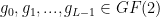
Key focus: Model and simulate m-sequence generator using Galois linear feedback shift registers (LFSR) that implement linear recursion. Plot correlation properties.
Maximum-length sequences (also called as m-sequences or pseudo random (PN) sequences) are constructed based on Galois field theory which is an extensive topic in itself. A detailed treatment on the subject of Galois field theory can be found in references [1] and [2].
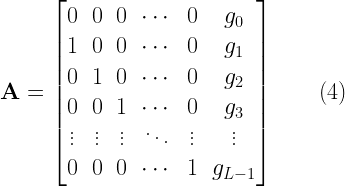
Maximum length sequences are generated using linear feedback shift registers(LFSR) structures that implement linear recursion. There are two types of LFSR structures available for implementation – 1) Galois LFSR and 2) Fibonacci LFSR. The Galois LFSR structure is a high speed implementation structure, since it has less clock to clock delay path compared to its Fibonacci equivalent. What follows in this discussion is the implementation of an m-sequence generator based on Galois LFSR architecture (Figure 1).
Figure 1: A basic LFSR architecture (m-sequence generator)
The basic Galois LFSR architecture for an -order generating polynomial in is given in Figure 1. The integer value denotes the number of delay elements in the LFSR architecture and represent the coefficients of the generator polynomial. The generator polynomial of the given LFSR is
where, , i.e, they take only binary values. The first and last coefficients are usually unity: .
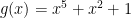
For generating an m-sequence, the characteristic polynomial that dictates the feedback coefficients, should be a primitive polynomial. Table 1 lists some of the primitive polynomials of degree upto . More comprehensive tables of primitive polynomials can be found in reference [3].
Table 1: Primitive polynomials up to degree L=12 used in m-sequence generator
For implementation in Matlab, the LFSR structure can be coded in a straightforward manner that involves at least two for loops. If we could exploit the linear recursion property of LFSR and its equivalent matrix model, the LFSR can be implemented using only one for loop as shown in the Matlab function given in the book (click here). The function implements the LFSR structure Figure 1 by using the following equivalent matrix equation:
with the initial state of the shift registers represented by the vector , and is an dimensional vector given by
Let’s generate an m-sequence of period using the order characteristic polynomial . The coefficients of the characteristic polynomial is and let’s start the generator with initial seed . Typically, the autocorrelation function of m-sequences are two valued. The normalized autocorrelation of an m-sequence of length , takes two values . This is demonstrated in Figure 2. We observe that that autocorrelation of m-sequence carries some similarities with that of a random sequence. If the length of the m-sequence is increased, the out-of-peak correlation reduces further and thereby the peaks become more distinct. This property makes the m-sequences suitable for synchronization and in the detection of information in single-user Direct Sequence Spread Spectrum systems.
Figure 2: Normalized autocorrelation of m-sequence generated using the polynomial
To demonstrate cross-correlation properties of two different m-sequences, consider two different primitive polynomials and that could generate two different m-sequences of length . The normalized cross-correlation of the aforementioned m-sequences, shown in Figure 3, is given by the Matlab script given in the book (click here).
The cross-correlation plot contains high peaks at certain lags (as high as ) and hence the m-sequences causes multiple access interference↗ (MAI), leading to severe performance degradation. Hence, the m-sequences are not suitable for orthogonalization of users in multi-user spread spectrum systems like CDMA.
Spread spectrum techniques
● Introduction
● Code sequences
□ Sequence correlations
□ Maximum-length sequences (m-sequences)
□ Gold codes
● Direct Sequence Spread Spectrum
□ Simulation of DSSS system
□ Performance of Direct Sequence Spread Spectrum over AWGN channel
□ Performance of Direct Sequence Spread spectrum in the presence of Jammer
● Frequency Hopping Spread Spectrum
□ Simulation model
□ Binary Frequency Shift Keying (BFSK)
□ Allocation of frequency channels
□ Frequency hopping generator
□ Fast and slow frequency hopping
□ Simulation code for BFSK-FHSS
In coherent detection, the receiver derives its demodulation frequency and phase references using a carrier synchronization loop. Such synchronization circuits may introduce phase ambiguity in the detected phase, which could lead to erroneous decisions in the demodulated bits. For example, Costas loop exhibits phase ambiguity of integral multiples of radians at the lock-in points. As a consequence, the carrier recovery may lock in radians out-of-phase thereby leading to a situation where all the detected bits are completely inverted when compared to the bits during perfect carrier synchronization. Phase ambiguity can be efficiently combated by applying differential encoding at the BPSK modulator input (Figure 1) and by performing differential decoding at the output of the coherent demodulator at the receiver side (Figure 2).
In ordinary BPSK transmission, the information is encoded as absolute phases: for binary 1 and for binary 0. With differential encoding, the information is encoded as the phase difference between two successive samples. Assuming is the message bit intended for transmission, the differential encoded output is given as
The differentially encoded bits are then BPSK modulated and transmitted. On the receiver side, the BPSK sequence is coherently detected and then decoded using a differential decoder. The differential decoding is mathematically represented as
This method can deal with the phase ambiguity introduced by synchronization circuits. However, it suffers from performance penalty due to the fact that the differential decoding produces wrong bits when: a) the preceding bit is in error and the present bit is not in error , or b) when the preceding bit is not in error and the present bit is in error. After differential decoding, the average bit error rate of coherently detected BPSK over AWGN channel is given by
Figure 2: Coherent detection of differentially encoded BPSK signal
Following is the Matlab implementation of the waveform simulation model for the method discussed above. Both the differential encoding and differential decoding blocks, illustrated in Figures 1 and 2, are linear time-invariant filters. The differential encoder is realized using IIR type digital filter and the differential decoder is realized as FIR filter.
File 1: dbpsk_coherent_detection.m: Coherent detection of D-BPSK over AWGN channel
Figure 3 shows the simulated BER points together with the theoretical BER curves for differentially encoded BPSK and the conventional coherently detected BPSK system over AWGN channel.
Key focus: Demodulation of phase modulated signal by extracting instantaneous phase can be done using Hilbert transform. Hands-on demo in Python & Matlab.
Phase modulated signal:
The concept of instantaneous amplitude/phase/frequency are fundamental to information communication and appears in many signal processing application. We know that a monochromatic signal of form x(t) = a cos(ω t + ɸ) cannot carry any information. To carry information, the signal need to be modulated. Different types of modulations can be performed – amplitude modulation, phase modulation / frequency modulation.
In amplitude modulation, the information is encoded as variations in the amplitude of a carrier signal. Demodulation of an amplitude modulated signal, involves extraction of envelope of the modulated signal. This was discussed and demonstrated here.
In phase modulation, the information is encoded as variations in the phase of the carrier signal. In its generic form, a phase modulated signal is expressed as an information-bearing sinusoidal signal modulating another sinusoidal carrier signal
\[x(t) = A cos \left[ 2 \pi f_c t + \beta + \alpha sin \left( 2 \pi f_m t + \theta \right) \right] \quad \quad \quad (1)\]
where, m(t) = α sin (2 π fm t + θ ) represents the information-bearing modulating signal, with the following parameters
α – amplitude of the modulating sinusoidal signal fm – frequency of the modulating sinusoidal signal θ – phase offset of the modulating sinusoidal signal
The carrier signal has the following parameters
A – amplitude of the carrier fc – frequency of the carrier and fc>>fm β – phase offset of the carrier
Demodulating a phase modulated signal:
The phase modulated signal shown in equation (1), can be simply expressed as
\[x(t) = A cos \left[ \phi(t) \right] \quad\quad\quad (2) \]
Here, ɸ(t) is the instantaneous phase that varies according to the information signal m(t).
A phase modulated signal of form x(t) can be demodulated by forming an analytic signal by applying Hilbert transform and then extracting the instantaneous phase. This method is explained here.
We note that the instantaneous phase is ɸ(t) = 2 π fc t + β + α sin (2 π fm t + θ) is linear in time, that is proportional to 2 π fc t . This linear offset needs to be subtracted from the instantaneous phase to obtained the information bearing modulated signal. If the carrier frequency is known at the receiver, this can be done easily. If not, the carrier frequency term 2 π fc t needs to be estimated using a linear fitof the unwrapped instantaneous phase. The following Matlab and Python codes demonstrate all these methods.
Matlab code
%Demonstrate simple Phase Demodulation using Hilbert transform
clearvars; clc;
fc = 240; %carrier frequency
fm = 10; %frequency of modulating signal
alpha = 1; %amplitude of modulating signal
theta = pi/4; %phase offset of modulating signal
beta = pi/5; %constant carrier phase offset
receiverKnowsCarrier= 'False'; %If receiver knows the carrier frequency & phase offset

fs = 8*fc; %sampling frequency
duration = 0.5; %duration of the signal
t = 0:1/fs:1-1/fs; %time base

%Phase Modulation
m_t = alpha*sin(2*pi*fm*t + theta); %modulating signal
x = cos(2*pi*fc*t + beta + m_t ); %modulated signal

figure(); subplot(2,1,1)
plot(t,m_t) %plot modulating signal
title('Modulating signal'); xlabel('t'); ylabel('m(t)')

subplot(2,1,2)
plot(t,x) %plot modulated signal
title('Modulated signal'); xlabel('t');ylabel('x(t)')

%Add AWGN noise to the transmitted signal
nMean = 0; %noise mean
nSigma = 0.1; %noise sigma
n = nMean + nSigma*randn(size(t)); %awgn noise
r = x + n;  %noisy received signal

%Demodulation of the noisy Phase Modulated signal
z= hilbert(r); %form the analytical signal from the received vector
inst_phase = unwrap(angle(z)); %instaneous phase

%If receiver don't know the carrier, estimate the subtraction term
if strcmpi(receiverKnowsCarrier,'True')
    offsetTerm = 2*pi*fc*t+beta; %if carrier frequency & phase offset is known
else
    p = polyfit(t,inst_phase,1); %linearly fit the instaneous phase
    estimated = polyval(p,t); %re-evaluate the offset term using the fitted values
    offsetTerm = estimated;
end

demodulated = inst_phase - offsetTerm;

figure()
plot(t,demodulated); %demodulated signal
title('Demodulated signal'); xlabel('n'); ylabel('\hat{m(t)}');
Python code
import numpy as np
from scipy.signal import hilbert
import matplotlib.pyplot as plt
PI = np.pi

fc = 240 #carrier frequency
fm = 10 #frequency of modulating signal
alpha = 1 #amplitude of modulating signal
theta = PI/4 #phase offset of modulating signal
beta = PI/5 #constant carrier phase offset
receiverKnowsCarrier= False; #If receiver knows the carrier frequency & phase offset

fs = 8*fc #sampling frequency
duration = 0.5 #duration of the signal
t = np.arange(int(fs*duration)) / fs #time base

#Phase Modulation
m_t = alpha*np.sin(2*PI*fm*t + theta) #modulating signal
x = np.cos(2*PI*fc*t + beta + m_t ) #modulated signal

plt.figure()
plt.subplot(2,1,1)
plt.plot(t,m_t) #plot modulating signal
plt.title('Modulating signal')
plt.xlabel('t')
plt.ylabel('m(t)')
plt.subplot(2,1,2)
plt.plot(t,x) #plot modulated signal
plt.title('Modulated signal')
plt.xlabel('t')
plt.ylabel('x(t)')

#Add AWGN noise to the transmitted signal
nMean = 0 #noise mean
nSigma = 0.1 #noise sigma
n = np.random.normal(nMean, nSigma, len(t))
r = x + n  #noisy received signal

#Demodulation of the noisy Phase Modulated signal
z= hilbert(r) #form the analytical signal from the received vector
inst_phase = np.unwrap(np.angle(z))#instaneous phase

#If receiver don't know the carrier, estimate the subtraction term
if receiverKnowsCarrier:
    offsetTerm = 2*PI*fc*t+beta; #if carrier frequency & phase offset is known
else:
    p = np.poly1d(np.polyfit(t,inst_phase,1)) #linearly fit the instaneous phase
    estimated = p(t) #re-evaluate the offset term using the fitted values
    offsetTerm = estimated

demodulated = inst_phase - offsetTerm

plt.figure()
plt.plot(t,demodulated) #demodulated signal
plt.title('Demodulated signal')
plt.xlabel('n')
plt.ylabel('\hat{m(t)}')
Results
Figure 1: Phase modulation – modulating signal and modulated (transmitted) signal
Key focus: Learn how to use Hilbert transform to extract envelope, instantaneous phase and frequency from a modulated signal. Hands-on demo using Python & Matlab.
The concept of instantaneous amplitude/phase/frequency are fundamental to information communication and appears in many signal processing application. We know that a monochromatic signal of form cannot carry any information. To carry information, the signal need to be modulated. Take for example the case of amplitude modulation, in which a positive real-valued signal modulates a carrier . That is, the amplitude modulation is effected by multiplying the information bearing signal with the carrier signal .
Here, is the angular frequency of the signal measured in radians/sec and is related to the temporal frequency as . The term is also called instantaneous amplitude.
Similarly, in the case of phase or frequency modulations, the concept of instantaneous phase or instantaneous frequency is required for describing the modulated signal.
Here, is the constant amplitude factor (no change in the envelope of the signal) and is the instantaneous phase which varies according to the information. The instantaneous angular frequency is expressed as the derivative of instantaneous phase.
Generalizing these concepts, if a signal is expressed as
The instantaneous amplitude or the envelope of the signal is given by
The instantaneous phase is given by
The instantaneous angular frequency is derived as
The instantaneous temporal frequency is derived as
Problem statement
An amplitude modulated signal is formed by multiplying a sinusoidal information and a linear frequency chirp. The information content is expressed as and the linear frequency chirp is made to vary from to . Given the modulated signal, extract the instantaneous amplitude (envelope), instantaneous phase and the instantaneous frequency.
Solution
We note that the modulated signal is a real-valued signal. We also take note of the fact that amplitude/phase and frequency can be easily computed if the signal is expressed in complex form. Which transform should we use such that the we can convert a real signal to the complex plane without altering the required properties ?? Answer: Apply Hilbert transform and form the analytic signal on the complex plane. Figure 1 illustrates this concept.
Figure 1: Converting a real-valued signal to complex plane using Hilbert Transform
If we express the real-valued modulated signal as an analytic signal, it is expressed in complex plane as
where, (HT[.]) represents the Hilbert Transform operation. Now, the required parameters are very easy to obtain.
The instantaneous amplitude (envelope extraction) is computed in the complex plane as
The instantaneous phase is computed in the complex plane as
The instantaneous temporal frequency is computed in the complex plane as
Once we know the instantaneous phase, the carrier can be regenerated as . The regenerated carrier is often referred as Temporal Fine Structure (TFS) in Acoustic signal processing [1].
Matlab
fs = 600; %sampling frequency in Hz
t = 0:1/fs:1-1/fs; %time base
a_t = 1.0 + 0.7 * sin(2.0*pi*3.0*t) ; %information signal
c_t = chirp(t,20,t(end),80); %chirp carrier
x = a_t .* c_t; %modulated signal

subplot(2,1,1); plot(x);hold on; %plot the modulated signal

z = hilbert(x); %form the analytical signal
inst_amplitude = abs(z); %envelope extraction
inst_phase = unwrap(angle(z));%inst phase
inst_freq = diff(inst_phase)/(2*pi)*fs;%inst frequency

%Regenerate the carrier from the instantaneous phase
regenerated_carrier = cos(inst_phase);

plot(inst_amplitude,'r'); %overlay the extracted envelope
title('Modulated signal and extracted envelope'); xlabel('n'); ylabel('x(t) and |z(t)|');
subplot(2,1,2); plot(cos(inst_phase));
title('Extracted carrier or TFS'); xlabel('n'); ylabel('cos[\omega(t)]');
Python
import numpy as np
from scipy.signal import hilbert, chirp
import matplotlib.pyplot as plt

fs = 600.0 #sampling frequency
duration = 1.0 #duration of the signal
t = np.arange(int(fs*duration)) / fs #time base

a_t =  1.0 + 0.7 * np.sin(2.0*np.pi*3.0*t)#information signal
c_t = chirp(t, 20.0, t[-1], 80) #chirp carrier
x = a_t * c_t #modulated signal

plt.subplot(2,1,1)
plt.plot(x) #plot the modulated signal

z= hilbert(x) #form the analytical signal
inst_amplitude = np.abs(z) #envelope extraction
inst_phase = np.unwrap(np.angle(z))#inst phase
inst_freq = np.diff(inst_phase)/(2*np.pi)*fs #inst frequency

#Regenerate the carrier from the instantaneous phase
regenerated_carrier = np.cos(inst_phase)

plt.plot(inst_amplitude,'r'); #overlay the extracted envelope
plt.title('Modulated signal and extracted envelope')
plt.xlabel('n')
plt.ylabel('x(t) and |z(t)|')
plt.subplot(2,1,2)
plt.plot(regenerated_carrier)
plt.title('Extracted carrier or TFS')
plt.xlabel('n')
plt.ylabel('cos[\omega(t)]')
Key focus of this article: Understand the relationship between analytic signal, Hilbert transform and FFT. Hands-on demonstration using Python and Matlab.
Introduction
Fourier Transform of a real-valued signal is complex-symmetric. It implies that the content at negative frequencies are redundant with respect to the positive frequencies. In their works, Gabor [1]and Ville [2], aimed to create an analytic signal by removing redundant negative frequency content resulting from the Fourier transform. The analytic signal is complex-valued but its spectrum will be one-sided (only positive frequencies) that preserved the spectral content of the original real-valued signal. Using an analytic signal instead of the original real-valued signal, has proven to be useful in many signal processing applications. For example, in spectral analysis, use of analytic signal in-lieu of the original real-valued signal mitigates estimation biases and eliminates cross-term artifacts due to negative and positive frequency components [3].
Let be a real-valued non-bandlimited finite energy signal, for which we wish to construct a corresponding analytic signal . The Continuous Time Fourier Transform of is given by
Lets say the magnitude spectrum of is as shown in Figure 1(a). We note that the signal is a real-valued and its magnitude spectrum is symmetric and extends infinitely in the frequency domain.
Figure 1: (a) Spectrum of continuous signal x(t) and (b) spectrum of analytic signal z(t)
As mentioned in the introduction, an analytic signal can be formed by suppressing the negative frequency contents of the Fourier Transform of the real-valued signal. That is, in frequency domain, the spectral content of the analytic signal is given by
The corresponding spectrum of the resulting analytic signal is shown in Figure 1(b).
Since the spectrum of the analytic signal is one-sided, the analytic signal will be complex valued in the time domain, hence the analytic signal can be represented in terms of real and imaginary components as . Since the spectral content is preserved in an analytic signal, it turns out that the real part of the analytic signal in time domain is essentially the original real-valued signal itself . Then, what takes place of the imaginary part ? Who is the companion to x(t) that occupies the imaginary part in the resulting analytic signal ? Summarizing as equation,
It is interesting to note that Hilbert transform [4]can be used to find a companion function (imaginary part in the equation above) to a real-valued signal such that the real signal can be analytically extended from the real axis to the upper half of the complex plane . Denoting Hilbert transform as , the analytic signal is given by
From these discussion, we can see that an analytic signal for a real-valued signal , can be constructed using two approaches.
● Frequency domain approach: The one-sided spectrum of is formed from the two-sided spectrum of the real-valued signal by applying equation (2) ● Time domain approach: Using Hilbert transform approach given in equation (4)
One of the important property of an analytic signal is that its real and imaginary components are orthogonal
Discrete-time analytic signal
Since we are in digital era, we are more interested in discrete-time signal processing. Consider a continuous real-valued signal gets sampled at interval seconds and results in real-valued discrete samples , i.e, . The spectrum of the continuous signal is shown in Figure 2(a). The spectrum of that results from the process of periodic sampling is given in Figure 2(b) (Refer here more details on the process of sampling). The spectrum of discrete-time signal can be obtained by Discrete-Time Fourier Transform (DTFT).
Figure 2: (a) CTFT of continuous signal x(t), (b) Spectrum of x[n] resulted due to periodic sampling and (c) Periodic one-sided spectrum of analytical signal z[n]
At this point, we would like to construct a discrete-time analytic signal from the real-valued sampled signal . We wish the analytic signal is complex valued and should satisfy the following two desired properties
● The real part of the analytic signal should be same as the original real-valued signal. ● The real and imaginary part of the analytic signal should satisfy the following property of orthogonality
In Frequency domain approach for the continuous-time case, we saw that an analytic signal is constructed by suppressing the negative frequency components from the spectrum of the real signal. We cannot do this for our periodically sampled signal . Periodic mirroring nature of the spectrum prevents one from suppressing the negative components. If we do so, it will vanish the entire spectrum. One solution to this problem is to set the negative half of each spectral period to zero. The resulting spectrum of the analytic signal is shown in Figure 2(c).
Given a record of samples of even length , the procedure to construct the analytic signal is as follows. This method satisfies both the desired properties listed above.
● Compute the -point DTFT of using FFT ● N-point periodic one-sided analytic signal is computed by the following transform
● Finally, the analytic signal (z[n]) is obtained by taking the inverse DTFT of
Matlab
The given procedure can be coded in Matlab using the FFT function. Given a record of real-valued samples , the corresponding analytic signal can be constructed as given next. Note that the Matlab has an inbuilt function to compute the analytic signal. The in-built function is called hilbert.
function z = analytic_signal(x)
%x is a real-valued record of length N, where N is even %returns the analytic signal z[n]
x = x(:); %serialize
N = length(x);
X = fft(x,N);
z = ifft([X(1); 2*X(2:N/2); X(N/2+1); zeros(N/2-1,1)],N);
end
To test this function, we create a 5 seconds record of a real-valued sine signal. The analytic signal is constructed and the orthogonal components are plotted in Figure 3. From the plot, we can see that the real part of the analytic signal is exactly same as the original signal (which is the cosine signal) and the imaginary part of the analytic signal is phase shifted version of the original signal. We note that the imaginary part of the analytic signal is a cosine function with amplitude scaled by which is none other than the Hilbert transform of sine function.
t=0:0.001:0.5-0.001;
x = sin(2*pi*10*t); %real-valued f = 10 Hz
subplot(2,1,1); plot(t,x);%plot the original signal
title('x[n] - original signal'); xlabel('n'); ylabel('x[n]');

z = analytic_signal(x); %construct analytic signal
subplot(2,1,2); plot(t, real(z), 'k'); hold on;
plot(t, imag(z), 'r');
title('Components of Analytic signal');
xlabel('n'); ylabel('z_r[n] and z_i[n]');
legend('Real(z[n])','Imag(z[n])');
Python
Equivalent code in Python is given below (tested with Python 3.6.0)
import numpy as np
def main():
    t = np.arange(start=0,stop=0.5,step=0.001)
    x = np.sin(2*np.pi*10*t)

    import matplotlib.pyplot as plt
    plt.subplot(2,1,1)
    plt.plot(t,x)
    plt.title('x[n] - original signal')
    plt.xlabel('n')
    plt.ylabel('x[n]')

    z = analytic_signal(x)

    plt.subplot(2,1,2)
    plt.plot(t,z.real,'k',label='Real(z[n])')
    plt.plot(t,z.imag,'r',label='Imag(z[n])')
    plt.title('Components of Analytic signal')
    plt.xlabel('n')
    plt.ylabel('z_r[n] and z_i[n]')
    plt.legend()

def analytic_signal(x):
    from scipy.fftpack import fft,ifft
    N = len(x)
    X = fft(x,N)
    h = np.zeros(N)
    h[0] = 1
    h[1:N//2] = 2*np.ones(N//2-1)
    h[N//2] = 1
    Z = X*h
    z = ifft(Z,N)
    return z

if __name__ == '__main__':
    main()
We should note that the hilbert function in Matlab returns the analytic signal $latex z[n]$ not the hilbert transform of the signal. To get the hilbert transform, we should simply get the imaginary part of the analytic signal. Since we have written our own function to compute the analytic signal, getting the hilbert transform of a real-valued signal goes like this.
A brief intro to modeling a frequency selective fading channel using tapped delay line (TDL) filters. Rayleigh & Rician frequency-selective fading channel models explained.
Tapped delay line filters
Tapped-delay line filters (FIR filters) are best to simulate multiple echoes originating from same source. Hence they can be used to model multipath scenarios. Tapped-Delay-Line (TDL) filters with number taps can be used to simulate a multipath frequency selective fading channel. Frequency selective channels are characterized by time varying nature of the channel. For simulating a frequency selective channel, it is mandatory to have N > 1. In contrast, if N = 1, it simulates a zero-mean fading channel where all the multipath signals arrive at the receiver at the same time.
Let be the associated path attenuation corresponding to the received power and propagation delay of the th path. In continuous time, the complex path attenuation is given by
The complex channel response is given by
In the equation above, the attenuation and path delay vary with time. This simulates a time-variant complex channel.
As a special case, in the absence any movements or other changes in the transmission channel, the channel can remain fairly time invariant (fixed channel with respect to instantaneous time ) even though the multipath is present. Thus the time-invariant complex channel becomes
Usually, the pair is described as a Power Delay Profile (PDP) plot. A sample power delay profile plot for a fixed, discrete, three ray model with its corresponding implementation using a tapped-delay line filter is shown in the following figure
Figure 1: 3-ray multipath time-invariant channel and its equivalent TDL implementation (path attenuations and propagation delays are fixed)
Choose underlying distribution:
The next level of modeling involves, introduction of randomness in the above mentioned model there by rendering the channel response time variant. If the path attenuations are typically drawn from a complex Gaussian random variable, then at any given time , the absolute value of the impulse response is
● Rayleigh distributed – if the mean of the distribution ● Rician distributed – if the mean of the distribution
Respectively, these two scenarios model the presence or absence of a Line of Sight (LOS) path between the transmitter and the receiver. The first propagation delay has no effect on the model behavior and hence it can be removed.
Similarly, the propagation delays can also be randomized, resulting in a more realistic but extremely complex model to implement. Furthermore, the power-delay-profile specifications with arbitrary time delays, warrant non-uniformly spaced tapped-delay-line filters, that are not suitable for practical simulation. For ease of implementation, the given PDP model with arbitrary time delays can be converted to tractable uniformly spaced statistical model by a combination of interpolation/approximation/uniform-sampling of the given power-delay-profile.
Real-life modelling:
Usually continuous domain equations for modeling multipath are specified in standards like COST-207 model in GSM specification. Such continuous time power-delay-profile models can be simulated using discrete-time Tapped Delay Line (TDL) filter with number of taps with variable tap gains. Given the order , the problem boils down to determining the discrete tap spacing and the path gains , in such a way that the simulated channel closely follows the specified multipath PDP characteristics. A survey of method to find a solution for this problem can be found in [2].
Rate this article: Note: There is a rating embedded within this post, please visit this post to rate it.
Small-scale Models for Multipath Effects
● Introduction
● Statistical characteristics of multipath channels
□ Mutipath channel models
□ Scattering function
□ Power delay profile
□ Doppler power spectrum
□ Classification of small-scale fading
● Rayleigh and Rice processes
□ Probability density function of amplitude
□ Probability density function of frequency
● Modeling frequency flat channel
● Modeling frequency selective channel
□ Method of equal distances (MED) to model specified power delay profiles
□ Simulating a frequency selective channel using TDL model
Key focus: With examples, let’s estimate and plot the probability density function of a random variable using Matlab histogram function.
Generation of random variables with required probability distribution characteristic is of paramount importance in simulating a communication system. Let’s see how we can generate a simple random variable, estimate and plot the probability density function (PDF) from the generated data and then match it with the intended theoretical PDF. Normal random variable is considered here for illustration. Other types of random variables like uniform, Bernoulli, binomial, Chi-squared, Nakagami-m are illustrated in the next section.
A survey of commonly used fundamental methods to generate a given random variable is given in [1]. For this demonstration, we will consider the normal random variable with the following parameters : – mean and – standard deviation. First generate a vector of randomly distributed random numbers of sufficient length (say 100000) with some valid values for and . There are more than one way to generate this. Some of them are given below.
● Method 1: Using the in-built random function (requires statistics toolbox)
mu=0;sigma=1;%mean=0,deviation=1
L=100000; %length of the random vector
R = random('Normal',mu,sigma,L,1);%method 1
● Method 2: Using randn function that generates normally distributed random numbers having and = 1
mu=0;sigma=1;%mean=0,deviation=1
L=100000; %length of the random vector
R = randn(L,1)*sigma + mu; %method 2
● Method 3: Box-Muller transformation [2] method using rand function that generates uniformly distributed random numbers
 mu=0;sigma=1;%mean=0,deviation=1
L=100000; %length of the random vector
U1 = rand(L,1); %uniformly distributed random numbers U(0,1)
U2 = rand(L,1); %uniformly distributed random numbers U(0,1)
Z = sqrt(-2log(U1)).cos(2piU2);%Standard Normal distribution
R = Z*sigma+mu;%Normal distribution with mean and sigma
Step 2: Plot the estimated histogram
Typically, if we have a vector of random numbers that is drawn from a distribution, we can estimate the PDF using the histogram tool. Matlab supports two in-built functions to compute and plot histograms:
● hist – introduced before R2006a ● histogram – introduced in R2014b
Which one to use ? Matlab’s help page points that the histfunction is notrecommended for several reasons and the issue of inconsistency is one among them. The histogram function is the recommended function to use.
Estimate and plot the normalized histogram using the recommended ‘histogram’ function. And for verification, overlay the theoretical PDF for the intended distribution. When using the histogram function to plot the estimated PDF from the generated random data, use ‘pdf’ option for ‘Normalization’ option. Do not use the ‘probability’ option for ‘Normalization’ option, as it will not match the theoretical PDF curve.
histogram(R,'Normalization','pdf'); %plot estimated pdf from the generated data

X = -4:0.1:4; %range of x to compute the theoretical pdf
fx_theory = pdf('Normal',X,mu,sigma); %theoretical normal probability density
hold on; plot(X,fx_theory,'r'); %plot computed theoretical PDF
title('Probability Density Function'); xlabel('values - x'); ylabel('pdf - f(x)'); axis tight;
legend('simulated','theory');
Estimated PDF (using histogram function) and the theoretical PDF
However, if you do not have Matlab version that was released before R2014b, use the ‘hist’ function and get the histogram frequency counts () and the bin-centers (). Using these data, normalize the frequency counts using the overall area under the histogram. Plot this normalized histogram and overlay the theoretical PDF for the chosen parameters.
%For those who don't have access to 'histogram' function
%get un-normalized values from hist function with same number of bins as histogram function
numBins=50; %choose appropriately
[f,x]=hist(R,numBins); %use hist function and get unnormalized values
figure; plot(x,f/trapz(x,f),'b-*');%plot normalized histogram from the generated data

X = -4:0.1:4; %range of x to compute the theoretical pdf
fx_theory =   pdf('Normal',X,mu,sigma); %theoretical normal probability density
hold on; plot(X,fx_theory,'r'); %plot computed theoretical PDF
title('Probability Density Function'); xlabel('values - x'); ylabel('pdf - f(x)'); axis tight;
legend('simulated','theory');
The given code snippets above, already include the command to plot the theoretical PDF by using the ‘pdf’ function in Matlab. It you do not have access to this function, you could use the following equation for computing the theoretical PDF
The code snippet for that purpose is given next.
X = -4:0.1:4; %range of x to compute the theoretical pdf
fx_theory = 1/sqrt(2*pi*sigma^2)*exp(-0.5*(X-mu).^2./sigma^2);
plot(X,fx_theory,'k'); %plot computed theoretical PDF
Note: The functions – ‘random’ and ‘pdf’ , requires statistics toolbox.
Rate this article: Note: There is a rating embedded within this post, please visit this post to rate it.
Synopsis: Cyclic prefix in OFDM, tricks a natural channel to perform circular convolution. This simplifies equalizer design at the receiver. Hands-on demo in Matlab.
Cyclic Prefix-ed OFDM
A cyclic-prefixed OFDM(CP-OFDM) transceiver architecture is typically implemented using inverse discrete Fourier transform (IDFT) and discrete Fourier transform (DFT) blocks (refer Figure 13.3). In an OFDM transmitter, the modulated symbols are assigned to individual subcarriers and sent to an IDFT block. The output of the IDFT block, generally viewed as time domain samples, results in an OFDM symbol. Such OFDM symbols are then transmitted across a channel with certain channel impulse response (CIR). On the other hand, the receiver applies DFT over the received OFDM symbols for further demodulation of the information in the individual subcarriers.
In reality, a multipath channel or any channel in nature acts as a linear filter on the transmitted OFDM symbols. Mathematically, the transmitted OFDM symbol (denoted as gets linearly convolved with the CIR and gets corrupted with additive white gaussian noise – designated as . Denoting linear convolution as ‘‘, the received signal in discrete-time can be represented as
The idea behind using OFDM is to combat frequency selective fading, where different frequency components of a transmitted signal can undergo different levels of fading. The OFDM divides the available spectrum in to small chunks called sub-channels. Within the subchannels, the fading experienced by the individual modulated symbol can be considered flat. This opens-up the possibility of using a simple frequency domain equalizer to neutralize the channel effects in the individual subchannels.
Circular convolution and designing a simple frequency domain equalizer
From one of the DFT properties, we know that the circular convolution of two sequences in time domain is equivalent to the multiplication of their individual responses in frequency domain.
Let and are two sequences of length with their DFTs denoted as and respectively. Denoting circular convolution as ,
If we ignore channel noise in the OFDM transmission, the received signal is written as
We can note that the channel performs a linear convolution operation on the transmitted signal. Instead, if the channel performs circular convolution (which is not the case in nature) then the equation would have been
By applying the DFT property given in equation 2,
As a consequence, the channel effects can be neutralized at the receiver using a simple frequency domain equalizer (actually this is a zero-forcing equalizer when viewed in time domain) that just inverts the estimated channel response and multiplies it with the frequency response of the received signal to obtain the estimates of the OFDM symbols in the subcarriers as
Demonstrating the role of Cyclic Prefix
The simple frequency domain equalizer shown in equation 6 is possible only if the channel performs circular convolution. But in nature, all channels perform linear convolution. The linear convolution can be converted into circular convolution by adding Cyclic Prefix (CP) in the OFDM architecture. The addition of CP makes the linear convolution imparted by the channel appear as circular convolution to the DFT process at the receiver (Reference [1]).
Let’s understand this by demonstration.
To simply stuffs, we will create two randomized vectors for and . is of length , the channel impulse response is of length and we intend to use -point DFT/IDFT wherever applicable.
N=8; %period of DFT
s = randn(1,8);
h = randn(1,3);
>> s =   -0.0155    2.5770    1.9238   -0.0629   -0.8105    0.6727   -1.5924   -0.8007
>> h =   -0.4878   -1.5351    0.2355
Now, convolve the vectors and linearly and circularly. The outputs are plotted in Figure 1. We note that the linear convolution and the circular convolution does not yield identical results.
lin_s_h = conv(h,s) %linear convolution of h and s
cir_s_h = cconv(h,s,N) % circular convolution of h and s with period N
Figure 1: Difference between linear convolution and circular convolution
Let’s append a cyclic prefix to the signal by copying last symbols from and pasting it to its front. Since the channel delay is 3 symbols (CIR of length 3), we need to add atleast 2 CP symbols.
Ncp = 2; %number of symbols to copy and paste for CP
s_cp = [s(end-Ncp+1:end) s]; %copy last Ncp symbols from s and prefix it.
Compare the outputs due to cir_s_h and lin_scp_h. We can immediately recognize that that the middle section of lin_scp_h is exactly same as the cir_s_h vector. This is shown in the figure 2.
We have just tricked the channel to perform circular convolution by adding a cyclic extension to the OFDM symbol. At the receiver, we are only interested in the middle section of the lin_scp_h which is the channel output. The first block in the OFDM receiver removes the additional symbols from the front and back of the channel output. The resultant vector is the received symbol r after the removal of cyclic prefix in the receiver.
r = lin_scp_h(Ncp+1:N+Ncp)%cut from index Ncp+1 to N+Ncp
Verifying DFT property
The DFT property given in equation 5 can be re-written as
To verify this in Matlab, take N-point DFTs of the received signal and CIR. Then, we can see that the IDFT of product of DFTs of and will be equal to the N-point circular convolution of and
R = fft(r,N); %frequency response of received signal
H = fft(h,N); %frequency response of CIR
S = fft(s,N); %frequency response of OFDM signal (non CP)

r1 = ifft(S.*H); %IFFT of product of individual DFTs

display(['IFFT(DFT(H)*DFT(S)) : ',num2str(r1)])
display([cconv(s,h): ', numstr(r)])
In the previous post, Interpretation of frequency bins, frequency axis arrangement (fftshift/ifftshift) for complex DFT were discussed. In this post, I intend to show you how to interpret FFT results and obtain magnitude and phase information.
Outline
For the discussion here, lets take an arbitrary cosine function of the form \(x(t)= A cos \left(2 \pi f_c t + \phi \right)\) and proceed step by step as follows
● Represent the signal \(x(t)\) in computer (discrete-time) and plot the signal (time domain) ● Represent the signal in frequency domain using FFT (\( X[k]\)) ● Extract amplitude and phase information from the FFT result ● Reconstruct the time domain signal from the frequency domain samples
Consider a cosine signal of amplitude \(A=0.5\), frequency \(f_c=10 Hz\) and phase \(phi= \pi/6\) radians (or \(30^{\circ}\) )
\[x(t) = 0.5 cos \left( 2 \pi 10 t + \pi/6 \right)\]
In order to represent the continuous time signal \(x(t)\) in computer memory, we need to sample the signal at sufficiently high rate (according to Nyquist sampling theorem). I have chosen a oversampling factor of \(32\) so that the sampling frequency will be \(f_s = 32 \times f_c \), and that gives \(640\) samples in a \(2\) seconds duration of the waveform record.
A = 0.5; %amplitude of the cosine wave
fc=10;%frequency of the cosine wave
phase=30; %desired phase shift of the cosine in degrees
fs=32*fc;%sampling frequency with oversampling factor 32
t=0:1/fs:2-1/fs;%2 seconds duration

phi = phase*pi/180; %convert phase shift in degrees in radians
x=A*cos(2*pi*fc*t+phi);%time domain signal with phase shift

figure; plot(t,x); %plot the signal
Represent the signal in frequency domain using FFT
Lets represent the signal in frequency domain using the FFT function. The FFT function computes \(N\)-point complex DFT. The length of the transformation \(N\) should cover the signal of interest otherwise we will some loose valuable information in the conversion process to frequency domain. However, we can choose a reasonable length if we know about the nature of the signal.
For example, the cosine signal of our interest is periodic in nature and is of length \(640\) samples (for 2 seconds duration signal). We can simply use a lower number \(N=256\) for computing the FFT. In this case, only the first \(256\) time domain samples will be considered for taking FFT. No need to worry about loss of information in this case, as the \(256\) samples will have sufficient number of cycles using which we can calculate the frequency information.
N=256; %FFT size
X = 1/N*fftshift(fft(x,N));%N-point complex DFT
In the code above, \(fftshift\) is used only for obtaining a nice double-sided frequency spectrum that delineates negative frequencies and positive frequencies in order. This transformation is not necessary. A scaling factor \(1/N\) was used to account for the difference between the FFT implementation in Matlab and the text definition of complex DFT.
3a. Extract amplitude of frequency components (amplitude spectrum)
The FFT function computes the complex DFT and the hence the results in a sequence of complex numbers of form \(X_{re} + j X_{im}\). The amplitude spectrum is obtained
\[|X[k]| = \sqrt{X_{re}^2 + X_{im}^2 } \]
For obtaining a double-sided plot, the ordered frequency axis (result of fftshift) is computed based on the sampling frequency and the amplitude spectrum is plotted.
df=fs/N; %frequency resolution
sampleIndex = -N/2:N/2-1; %ordered index for FFT plot
f=sampleIndex*df; %x-axis index converted to ordered frequencies
stem(f,abs(X)); %magnitudes vs frequencies
xlabel('f (Hz)'); ylabel('|X(k)|');
3b. Extract phase of frequency components (phase spectrum)
Extracting the correct phase spectrum is a tricky business. I will show you why it is so. The phase of the spectral components are computed as
That equation looks naive, but one should be careful when computing the inverse tangents using computers. The obvious choice for implementation seems to be the \(atan\) function in Matlab. However, usage of \(atan\) function will prove disastrous unless additional precautions are taken. The \(atan\) function computes the inverse tangent over two quadrants only, i.e, it will return values only in the \([-\pi/2 , \pi/2]\) interval. Therefore, the phase need to be unwrapped properly. We can simply fix this issue by computing the inverse tangent over all the four quadrants using the \(atan2(X_{img},X_{re})\) function.
Lets compute and plot the phase information using \(atan2\) function and see how the phase spectrum looks
phase=atan2(imag(X),real(X))*180/pi; %phase information
plot(f,phase); %phase vs frequencies
The phase spectrum is completely noisy. Unexpected !!!. The phase spectrum is noisy due to fact that the inverse tangents are computed from the \(ratio\) of imaginary part to real part of the FFT result. Even a small floating rounding off error will amplify the result and manifest incorrectly as useful phase information (read how a computer program approximates very small numbers).
To understand, print the first few samples from the FFT result and observe that they are not absolute zeros (they are very small numbers in the order \(10^{-16}\). Computing inverse tangent will result in incorrect results.
The solution is to define a tolerance threshold and ignore all the computed phase values that are below the threshold.
X2=X;%store the FFT results in another array
%detect noise (very small numbers (eps)) and ignore them
threshold = max(abs(X))/10000; %tolerance threshold
X2(abs(X)<threshold) = 0; %maskout values that are below the threshold
phase=atan2(imag(X2),real(X2))*180/pi; %phase information
plot(f,phase); %phase vs frequencies
The recomputed phase spectrum is plotted below. The phase spectrum has correctly registered the \(30^{\circ}\) phase shift at the frequency \(f=10 Hz\). The phase spectrum is anti-symmetric (\(\phi=-30^{\circ}\) at \(f=-10 Hz\) ), which is expected for real-valued signals.
Reconstruct the time domain signal from the frequency domain samples
Reconstruction of the time domain signal from the frequency domain sample is pretty straightforward
x_recon = N*ifft(ifftshift(X),N); %reconstructed signal
t = [0:1:length(x_recon)-1]/fs; %recompute time index
plot(t,x_recon);%reconstructed signal
The reconstructed signal has preserved the same initial phase shift and the frequency of the original signal. Note: The length of the reconstructed signal is only \(256\) sample long (\(\approx 0.8\) seconds duration), this is because the size of FFT is considered as \(N=256\). Since the signal is periodic it is not a concern. For more complicated signals, appropriate FFT length (better to use a value that is larger than the length of the signal) need to be used.
Rate this post: Note: There is a rating embedded within this post, please visit this post to rate it.
In this article, the relationship between SNR-per-bit (Eb/N0) and SNR-per-symbol (Es/N0) are defined with respect to M-ary signaling schemes. Then the complex baseband model for an AWGN channel is discussed, followed by the theoretical error rates of various modulations over the additive white Gaussian noise (AWGN) channel. Finally, the complex baseband models for digital modulators and detectors developed in previous chapter of this book, are incorporated to build a complete communication system model.
Assuming a channel of bandwidth B, received signal power Pr and the power spectral density (PSD) of noise N0/2, the signal to noise ratio (SNR) is given by
Let a signal’s energy-per-bit is denoted as Eb and the energy-per-symbol as Es, then γb=Eb/N0and γs=Es/N0 are the SNR-per-bit and the SNR-per-symbol respectively.
For uncoded M-ary signaling scheme with k = log2(M) bits per symbol, the signal energy per modulated symbol is given by
The SNR per symbol is given by
AWGN channel model
In order to simulate a specific SNR point in performance simulations, the modulated signal from the transmitter needs to be added with random noise of specific strength. The strength of the generated noise depends on the desired SNR level which usually is an input in such simulations. In practice, SNRs are specified in dB. Given a specific SNR point for simulation, let’s see how we can simulate an AWGN channel that adds correct level of white noise to the transmitted symbols.
Figure 1: Simplified simulation model for awgn channel
Consider the AWGN channel model given in Figure 1. Given a specific SNR point to simulate, we wish to generate a white Gaussian noise vector of appropriate strength and add it to the incoming signal. The method described can be applied for both waveform simulations and the complex baseband simulations. In following text, the term SNR (γ) refers to γb = Eb/N0 when the modulation is of binary type (example: BPSK). For multilevel modulations such as QPSK and MQAM, the term SNR refers to γs = Es/N0.
(1) Assume, s is a vector that represents the transmitted signal. We wish to generate a vector r that represents the signal after passing through the AWGN channel. The amount of noise added by the AWGN channel is controlled by the given SNR – γ
(3) Let N denotes the length of the vector s. The signal power for the vector s can be measured as,
(4) The required power spectral density of the noise vector n is computed as
(5) Assuming complex IQ plane for all the digital modulations, the required noise variance (noise power) for generating Gaussian random noise is given by
(6) Generate the noise vector n drawn from normal distribution with mean set to zero and the standard deviation computed from the equation given above
(7) Finally add the generated noise vector (n) to the signal (s)
Matlab code
The following custom function written in Matlab, can be used for adding AWGN noise to an incoming signal. It can be used in waveform simulation as well as complex baseband simulation models.
%author - Mathuranathan Viswanathan (gaussianwaves.com
%This code is part of the books: Wireless communication systems using Matlab & Digital modulations using Matlab.

function [r,n,N0] = add_awgn_noise(s,SNRdB,L)
%Function to add AWGN to the given signal
%[r,n,N0]= add_awgn_noise(s,SNRdB) adds AWGN noise vector to signal
%'s' to generate a %resulting signal vector 'r' of specified SNR
%in dB. It also returns the noise vector 'n' that is added to the
%signal 's' and the spectral density N0 of noise added
%
%[r,n,N0]= add_awgn_noise(s,SNRdB,L) adds AWGN noise vector to
%signal 's' to generate a resulting signal vector 'r' of specified
%SNR in dB. The parameter 'L' specifies the oversampling ratio used
%in the system (for waveform simulation). It also returns the noise
%vector 'n' that is added to the signal 's' and the spectral
%density N0 of noise added
 s_temp=s;
 if iscolumn(s), s=s.'; end; %to return the result in same dim as 's'
 gamma = 10ˆ(SNRdB/10); %SNR to linear scale

 if nargin==2, L=1; end %if third argument is not given, set it to 1

 if isvector(s),
  P=L*sum(abs(s).ˆ2)/length(s);%Actual power in the vector
 else %for multi-dimensional signals like MFSK
  P=L*sum(sum(abs(s).ˆ2))/length(s); %if s is a matrix [MxN]
 end

 N0=P/gamma; %Find the noise spectral density
 if(isreal(s)),
  n = sqrt(N0/2)*randn(size(s));%computed noise
 else
  n = sqrt(N0/2)*(randn(size(s))+1i*randn(size(s)));%computed noise
 end

 r = s + n; %received signal

 if iscolumn(s_temp), r=r.'; end;%return r in original format as s
end
Python code
The following custom function written in Python 3, can be used for adding AWGN noise to an incoming signal. It can be used in waveform simulation as well as complex baseband simulation models.
# author - Mathuranathan Viswanathan (gaussianwaves.com
# This code is part of the book Digital Modulations using Python

from numpy import sum,isrealobj,sqrt
from numpy.random import standard_normal

def awgn(s,SNRdB,L=1):
    """
    AWGN channel
    Add AWGN noise to input signal. The function adds AWGN noise vector to signal 's' to generate a resulting signal vector 'r' of specified SNR in dB. It also
    returns the noise vector 'n' that is added to the signal 's' and the power spectral density N0 of noise added
    Parameters:
        s : input/transmitted signal vector
        SNRdB : desired signal to noise ratio (expressed in dB) for the received signal
        L : oversampling factor (applicable for waveform simulation) default L = 1.
    Returns:
        r : received signal vector (r=s+n)
"""
    gamma = 10**(SNRdB/10) #SNR to linear scale
    if s.ndim==1:# if s is single dimensional vector
        P=L*sum(abs(s)**2)/len(s) #Actual power in the vector
    else: # multi-dimensional signals like MFSK
        P=L*sum(sum(abs(s)**2))/len(s) # if s is a matrix [MxN]
    N0=P/gamma # Find the noise spectral density
    if isrealobj(s):# check if input is real/complex object type
        n = sqrt(N0/2)*standard_normal(s.shape) # computed noise
    else:
        n = sqrt(N0/2)*(standard_normal(s.shape)+1j*standard_normal(s.shape))
    r = s + n # received signal
return r
Theoretical symbol error rates for digital modulations in AWGN channel
Denoting the symbol error rate (SER) as , SNR-per-bit as and SNR-per-symbol as , the symbol error rates for various modulation schemes over AWGN channel are listed in Table 1 (refer [1]).
Table 1: Theoretical symbol error rate for various modulations in AWGN channel
The theoretical symbol error rates are coded as a reusable function. In this implementation, erfc function is used instead of the Q function shown in the Table 4.1. The following equation describes the relationship between the erfc function and the Q function.
Unified simulation model for performance simulation
In the previous chapter of the books, the code implementation for complex baseband models for various digital modulators and demodulator are given. Using these models, we can create a unified simulation code for simulating the performance of various modulation techniques over AWGN channel.
The complete simulation model for performance simulation over AWGN channel is given in Figure 2. The figure is illustrated for a coherent communication system model (applicable for MPSK/MQAM/MPAM modulations)
Figure 2: Complete simulation model for a communication system with AWGN channel
The Matlab code implementing the aforementioned simulation model is given in the books. Here, an unified approach is employed to simulate the performance of any of the given modulation technique – MPSK, MQAM, MPAM or MFSK (MFSK simulation technique is available in the following books: Digital Modulations using Python and Digital Modulations using Matlab).
The simulation code will automatically choose the selected modulation type, performs Monte Carlo simulation, computes symbol error rates and plots them against the theoretical symbol error rates. The simulated performance results obtained for MQAM and MPSK modulations are shown in the Figure 3 and Figure 4.
Figure 3: Simulated symbol error rate performance of M-QAM modulation over AWGN channel
This website uses cookies to improve your experience while you navigate through the website. Out of these, the cookies that are categorized as necessary are stored on your browser as they are essential for the working of basic functionalities of the website. We also use third-party cookies that help us analyze and understand how you use this website. These cookies will be stored in your browser only with your consent. You also have the option to opt-out of these cookies. But opting out of some of these cookies may affect your browsing experience.
Necessary cookies are absolutely essential for the website to function properly. These cookies ensure basic functionalities and security features of the website, anonymously.
Cookie
Duration
Description
cookielawinfo-checbox-analytics
11 months
This cookie is set by GDPR Cookie Consent plugin. The cookie is used to store the user consent for the cookies in the category "Analytics".
cookielawinfo-checbox-analytics
11 months
This cookie is set by GDPR Cookie Consent plugin. The cookie is used to store the user consent for the cookies in the category "Analytics".
cookielawinfo-checbox-functional
11 months
The cookie is set by GDPR cookie consent to record the user consent for the cookies in the category "Functional".
cookielawinfo-checbox-functional
11 months
The cookie is set by GDPR cookie consent to record the user consent for the cookies in the category "Functional".
cookielawinfo-checbox-others
11 months
This cookie is set by GDPR Cookie Consent plugin. The cookie is used to store the user consent for the cookies in the category "Other.
cookielawinfo-checbox-others
11 months
This cookie is set by GDPR Cookie Consent plugin. The cookie is used to store the user consent for the cookies in the category "Other.
cookielawinfo-checkbox-necessary
11 months
This cookie is set by GDPR Cookie Consent plugin. The cookies is used to store the user consent for the cookies in the category "Necessary".
cookielawinfo-checkbox-performance
11 months
This cookie is set by GDPR Cookie Consent plugin. The cookie is used to store the user consent for the cookies in the category "Performance".
viewed_cookie_policy
11 months
The cookie is set by the GDPR Cookie Consent plugin and is used to store whether or not user has consented to the use of cookies. It does not store any personal data.
Functional cookies help to perform certain functionalities like sharing the content of the website on social media platforms, collect feedbacks, and other third-party features.
Performance cookies are used to understand and analyze the key performance indexes of the website which helps in delivering a better user experience for the visitors.
Analytical cookies are used to understand how visitors interact with the website. These cookies help provide information on metrics the number of visitors, bounce rate, traffic source, etc.


![G=[g_5,g_4,g_3,g_2,g_1,g_0]=[1,0,0,1,0,0]](https://s0.wp.com/latex.php?latex=G%3D%5Bg_5%2Cg_4%2Cg_3%2Cg_2%2Cg_1%2Cg_0%5D%3D%5B1%2C0%2C0%2C1%2C0%2C0%5D&bg=ffffff&fg=000&s=0&c=20201002)

![X_0=[0,0,0,0,1]](https://s0.wp.com/latex.php?latex=X_0%3D%5B0%2C0%2C0%2C0%2C1%5D&bg=ffffff&fg=000&s=0&c=20201002)


![[1,-1/N]](https://s0.wp.com/latex.php?latex=%5B1%2C-1%2FN%5D&bg=ffffff&fg=000&s=0&c=20201002)


![a[k]](https://s0.wp.com/latex.php?latex=a%5Bk%5D&bg=ffffff&fg=000&s=0&c=20201002)

![b[k] = b[k-1] \oplus a[k] \;\;\;\;\;\; (modulo-2) \;\;\;\;\;\; (1)](https://s0.wp.com/latex.php?latex=b%5Bk%5D+%3D+b%5Bk-1%5D+%5Coplus+a%5Bk%5D+%5C%3B%5C%3B%5C%3B%5C%3B%5C%3B%5C%3B+%28modulo-2%29+%5C%3B%5C%3B%5C%3B%5C%3B%5C%3B%5C%3B+%281%29+&bg=ffffff&fg=000&s=2&c=20201002)

![a[k] = b[k] \oplus b[k-1] \;\;\;\;\;\; (modulo-2) \;\;\;\;\;\; (2)](https://s0.wp.com/latex.php?latex=a%5Bk%5D+%3D+b%5Bk%5D+%5Coplus+b%5Bk-1%5D%C2%A0+%5C%3B%5C%3B%5C%3B%5C%3B%5C%3B%5C%3B+%28modulo-2%29+%5C%3B%5C%3B%5C%3B%5C%3B%5C%3B%5C%3B+%282%29+&bg=ffffff&fg=000&s=2&c=20201002)


![P_b = erfc \left(\sqrt{\frac{E_b}{N_0}} \right) \left[ 1-\frac{1}{2} erfc \left( \sqrt{\frac{E_b}{N_0}} \right) \right] \;\; (3)](https://s0.wp.com/latex.php?latex=P_b+%3D+erfc+%5Cleft%28%5Csqrt%7B%5Cfrac%7BE_b%7D%7BN_0%7D%7D+%5Cright%29+%5Cleft%5B+1-%5Cfrac%7B1%7D%7B2%7D+erfc+%5Cleft%28+%5Csqrt%7B%5Cfrac%7BE_b%7D%7BN_0%7D%7D+%5Cright%29+%5Cright%5D+%5C%3B%5C%3B+%283%29+&bg=ffffff&fg=000&s=2&c=20201002)


![x(t) = a(t) cos \left[ \phi (t) \right]](https://s0.wp.com/latex.php?latex=x%28t%29+%3D+a%28t%29+cos+%5Cleft%5B+%5Cphi+%28t%29+%5Cright%5D+&bg=ffffff&fg=000&s=0&c=20201002)


![z(t) = z_r(t) + j z_i(t) = x(t) + j HT \left[ x(t) \right]](https://s0.wp.com/latex.php?latex=z%28t%29+%3D+z_r%28t%29+%2B+j+z_i%28t%29+%3D+x%28t%29+%2B+j+HT+%5Cleft%5B+x%28t%29+%5Cright%5D+&bg=ffffff&fg=000&s=2&c=20201002)


![\phi(t) = \angle z(t) = arctan \left[ \frac{z_i(t)}{z_r(t)} \right]](https://s0.wp.com/latex.php?latex=%5Cphi%28t%29+%3D+%5Cangle+z%28t%29+%3D+arctan+%5Cleft%5B+%5Cfrac%7Bz_i%28t%29%7D%7Bz_r%28t%29%7D+%5Cright%5D+&bg=ffffff&fg=000&s=2&c=20201002)


![cos[\phi(t)]](https://s0.wp.com/latex.php?latex=cos%5B%5Cphi%28t%29%5D&bg=ffffff&fg=000&s=0&c=20201002)


![x[n]](https://s0.wp.com/latex.php?latex=x%5Bn%5D&bg=ffffff&fg=000&s=0&c=20201002)
![x[n] = x(nT)](https://s0.wp.com/latex.php?latex=x%5Bn%5D+%3D+x%28nT%29+&bg=ffffff&fg=000&s=0&c=20201002)

![X(f) = \displaystyle{ T \sum_{n=0}^{N-1} x[n] e^{-j 2 \pi f n T} }\quad (6)](https://s0.wp.com/latex.php?latex=X%28f%29+%3D+%5Cdisplaystyle%7B+T+%5Csum_%7Bn%3D0%7D%5E%7BN-1%7D+x%5Bn%5D+e%5E%7B-j+2+%5Cpi+f+n+T%7D+%7D%5Cquad+%286%29+%C2%A0&bg=ffffff&fg=000&s=2&c=20201002)

![(a) CTFT of continuous signal x(t), (b) Spectrum of x[n] resulted due to periodic sampling and (c) Periodic one-sided spectrum of analytical signal z[n]](https://i0.wp.com/www.gaussianwaves.com/gaussianwaves/wp-content/uploads/2017/04/discrete_time_analytic_signal_PNG.png?resize=594%2C494&ssl=1)
![z[n]](https://s0.wp.com/latex.php?latex=z%5Bn%5D&bg=ffffff&fg=000&s=0&c=20201002)
![z[n] = z_r[n] + j z_i[n]](https://s0.wp.com/latex.php?latex=z%5Bn%5D+%3D+z_r%5Bn%5D+%2B+j+z_i%5Bn%5D&bg=ffffff&fg=000&s=0&c=20201002)

![z_r[n] = x[n]](https://s0.wp.com/latex.php?latex=z_r%5Bn%5D+%3D+x%5Bn%5D&bg=ffffff&fg=000&s=0&c=20201002)

![\displaystyle{ \sum_{n=0}^{N-1} z_r[n] z_i[n] = 0 }](https://s0.wp.com/latex.php?latex=%5Cdisplaystyle%7B+%5Csum_%7Bn%3D0%7D%5E%7BN-1%7D+z_r%5Bn%5D+z_i%5Bn%5D+%3D+0+%7D++&bg=ffffff&fg=000&s=2&c=20201002)


![Z[m]](https://s0.wp.com/latex.php?latex=Z%5Bm%5D&bg=ffffff&fg=000&s=0&c=20201002)

![z[n] = \displaystyle{ \frac{1}{NT} \sum_{m=0}^{N-1} z[m] \; exp \left( j 2 \pi mn/N\right)}](https://s0.wp.com/latex.php?latex=z%5Bn%5D+%3D+%5Cdisplaystyle%7B+%5Cfrac%7B1%7D%7BNT%7D+%5Csum_%7Bm%3D0%7D%5E%7BN-1%7D+z%5Bm%5D+%5C%3B+exp+%5Cleft%28+j+2+%5Cpi+mn%2FN%5Cright%29%7D+&bg=ffffff&fg=000&s=2&c=20201002)


![\displaystyle{\tilde{a_n}(t) = a_n(t) exp\left[ -j 2 \pi f_c \tau_n(t) \right]}](https://s0.wp.com/latex.php?latex=%5Cdisplaystyle%7B%5Ctilde%7Ba_n%7D%28t%29+%3D+a_n%28t%29+exp%5Cleft%5B+-j+2+%5Cpi+f_c+%5Ctau_n%28t%29+%5Cright%5D%7D+&bg=ffffff&fg=000&s=2&c=20201002)


![E [h(t; \tau)] = 0](https://s0.wp.com/latex.php?latex=E+%5Bh%28t%3B+%5Ctau%29%5D+%3D+0&bg=ffffff&fg=000&s=0&c=20201002)
![E [h(t; \tau)] \neq 0](https://s0.wp.com/latex.php?latex=E+%5Bh%28t%3B+%5Ctau%29%5D+%5Cneq+0&bg=ffffff&fg=000&s=0&c=20201002)


![f_X(x) = \frac{1}{ \sqrt{ 2 \pi \sigma^2 }} exp \left[ -\frac{ \left( x-\mu \right) ^2}{2 \sigma^2} \right]](https://s0.wp.com/latex.php?latex=f_X%28x%29+%3D+%5Cfrac%7B1%7D%7B+%5Csqrt%7B+2+%5Cpi+%5Csigma%5E2+%7D%7D+exp+%5Cleft%5B+-%5Cfrac%7B+%5Cleft%28+x-%5Cmu+%5Cright%29+%5E2%7D%7B2+%5Csigma%5E2%7D+%5Cright%5D+&bg=ffffff&fg=000&s=2&c=20201002)
![s[n]](https://s0.wp.com/latex.php?latex=s%5Bn%5D&bg=ffffff&fg=000&s=0&c=20201002)
![h[n]](https://s0.wp.com/latex.php?latex=h%5Bn%5D&bg=ffffff&fg=000&s=0&c=20201002)

![w[n]](https://s0.wp.com/latex.php?latex=w%5Bn%5D&bg=ffffff&fg=000&s=0&c=20201002)


![r[n] = h[n] \ast s[n] + w[n] \;\;\; (\ast \rightarrow linear\;convolution ) \quad\quad (1)](https://s0.wp.com/latex.php?latex=r%5Bn%5D+%3D+h%5Bn%5D+%5Cast+s%5Bn%5D+%2B+w%5Bn%5D+%5C%3B%5C%3B%5C%3B+%28%5Cast+%5Crightarrow+linear%5C%3Bconvolution+%29+%5Cquad%5Cquad+%281%29+&bg=ffffff&fg=000&s=2&c=20201002)
![S[k]](https://s0.wp.com/latex.php?latex=S%5Bk%5D&bg=ffffff&fg=000&s=0&c=20201002)
![H[k]](https://s0.wp.com/latex.php?latex=H%5Bk%5D&bg=ffffff&fg=000&s=0&c=20201002)


![h[n] \circledast s[n] \equiv H[k] S[k] \quad\quad (2)](https://s0.wp.com/latex.php?latex=h%5Bn%5D+%5Ccircledast+s%5Bn%5D+%5Cequiv+H%5Bk%5D+S%5Bk%5D+%5Cquad%5Cquad+%282%29+&bg=ffffff&fg=000&s=2&c=20201002)

![r[n] = h[n] \ast s[n] \quad\quad (\ast \rightarrow linear\;convolution ) \quad\quad (3)](https://s0.wp.com/latex.php?latex=r%5Bn%5D+%3D+h%5Bn%5D+%5Cast+s%5Bn%5D+%5Cquad%5Cquad+%28%5Cast+%5Crightarrow+linear%5C%3Bconvolution+%29+%5Cquad%5Cquad+%283%29+&bg=ffffff&fg=000&s=2&c=20201002)

![r[n] = h[n] \circledast s[n] \quad\quad (\circledast \rightarrow circular\;convolution ) \quad\quad (4)](https://s0.wp.com/latex.php?latex=r%5Bn%5D+%3D+h%5Bn%5D+%5Ccircledast+s%5Bn%5D+%5Cquad%5Cquad+%28%5Ccircledast+%5Crightarrow+circular%5C%3Bconvolution+%29+%5Cquad%5Cquad+%284%29+&bg=ffffff&fg=000&s=2&c=20201002)

![r[n] = h[n] \circledast s[n] \quad\quad \equiv R[k] = H[k] S[k] \quad\quad (5)](https://s0.wp.com/latex.php?latex=r%5Bn%5D+%3D+h%5Bn%5D+%5Ccircledast+s%5Bn%5D+%5Cquad%5Cquad+%5Cequiv+R%5Bk%5D+%3D+H%5Bk%5D+S%5Bk%5D+%5Cquad%5Cquad+%285%29+&bg=ffffff&fg=000&s=2&c=20201002)

![\hat{S}[k] = \frac{R[k]}{H[k]} \quad\quad (6)](https://s0.wp.com/latex.php?latex=%5Chat%7BS%7D%5Bk%5D+%3D+%5Cfrac%7BR%5Bk%5D%7D%7BH%5Bk%5D%7D+%5Cquad%5Cquad+%286%29+&bg=ffffff&fg=000&s=2&c=20201002)


