In the previous post on Single Input Multiple Output (SIMO) models for receive diversity, various receiver diversity techniques were outlined. One of them is maximum ratio combining, the focus of the topic here.
Channel model
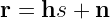
Assuming flat slow fading channel, the received signal model is given by

where,


Assuming small scale Rayleigh fading, the channel impulse response is modeled as complex Gaussian random variable with zero mean and variance


Therefore, the instantaneous channel power is exponentially distributed

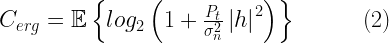
In the context of AWGN channel, the signal-to-noise ratio (SNR) for a given channel condition, is a constant. But in the case of fading channels, the signal-to-noise ratio is no longer a constant as the signal is fluctuating when passed through a fading channel. Therefore, for fading channel, the SNR has a random variable component built into it. Hence, we just don’t call it SNR, instead it is called instantaneous SNR which depends on the current conditions of the channel (or equivalently, the value of the random variable at that instant). Since the SNR is a random variable, we can also talk about its expected (average) value, which is called average SNR. Denoting the average SNR as


The instantaneous SNR


Therefore, like the channel impulse response, the instantaneous SNR is also exponentially distributed

Maximum Ratio Combining (MRC)
The selection combining technique is the simplest technique, where in, the received signal from the antenna that experiences the highest SNR (i.e, the strongest signal from N received signals) is chosen for processing at the receiver. Therefore this technique throws away


MRC works on the signal in spatial domain and is very similar to what a matched filter in frequency domain does to the incoming signal. MRC maximizes the inner product of the weights and the signal vector.


The maximum ratio combining technique, uses all the


With the weights set as


Therefore, the output SNR after MRC processing is

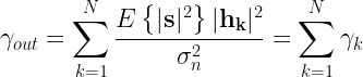
MRC processing results in the weighted average of the received signals and hence the overall output SNR is equal to the sum of the SNRs of all individual receive signals, which yields the maximum possible diversity gain of
Generally, two figures of merits are used to gauge the performance of the diversity schemes – outage probability and error rate performance for PSK modulation.
Outage probability
As we know, fading channels are characterized by deep fades, i.e, the period when the signal level falls below a certain threshold or certain noise level. During such fades, the user experiences signal outage. We would like to compute the probability, in certain fading channel, that a user will experience signal outage. This is called outage probability. Outage probability can be easily computed if we know the probability distribution characteristics of the fading.
The outage probability with which the instantaneous output SNR of MRC falls below a given SNR target


![P_{outage} = P \left[\gamma_{out} < \gamma_t \right] = 1 - e^{-\gamma_t/\Gamma} \sum_{n=0}^{N-1} \left( \frac{\gamma_t}{\Gamma} \right)^n \frac{1}{n!}](https://s0.wp.com/latex.php?latex=P_%7Boutage%7D+%3D+P+%5Cleft%5B%5Cgamma_%7Bout%7D+%3C+%5Cgamma_t+%5Cright%5D+%3D+1+-+e%5E%7B-%5Cgamma_t%2F%5CGamma%7D+%5Csum_%7Bn%3D0%7D%5E%7BN-1%7D+%5Cleft%28+%5Cfrac%7B%5Cgamma_t%7D%7B%5CGamma%7D+%5Cright%29%5En+%5Cfrac%7B1%7D%7Bn%21%7D+&bg=ffffff&fg=000&s=2&c=20201002)
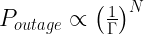
For high average SNR conditions


Python code
import numpy as np
import matplotlib.pyplot as plt
from scipy.special import factorial

gamma_ratio_dB = np.arange(start=-10,stop=40,step=2)
Ns = [1,2,3,4,10,20] #number of received signal paths

gamma_ratio = 10**(gamma_ratio_dB/10) #Average SNR/SNR threshold in dB

fig, ax = plt.subplots(1, 1)

for N in Ns:
        n = np.arange(start=0,stop=N,step=1)
        P_outage = 1 - np.exp(-1/gamma_ratio)*np.sum(((1/gamma_ratio)**n[:,None])/factorial(n[:,None]),axis=0)
        ax.semilogy(gamma_ratio_dB,P_outage,label='N='+str(N))

ax.legend()
ax.set_xlim(-10,40);ax.set_ylim(0.0001,1.1)
ax.set_title('MRC outage probability (Rayleigh fading channel)')
ax.set_xlabel(r'$10log_{10}\left(\Gamma/\gamma_t\right)$')
ax.set_ylabel('Outage probability');fig.show()


Figure 2, plots the outage probability against


Error rate performance
In the case of receive diversity schemes with

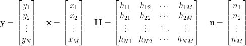
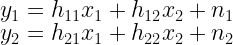
Considering the QPSK modulated symbols that are transmitted (denoted as


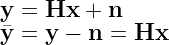
The solution to this problem can be obtained using the least squares method (refer equation 8.17 given in chapter 8 of this book)

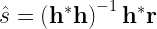
The solution can be re-written as


As an example, the symbol error rate performance of a QPSK modulated transmission over a Rayleigh flat fading SIMO channel, for a range of values for the number of receive antennas (
The code utilizes the modem class discussed in the book here. The modem class incorporates modulation and demodulation techniques for PSK,PAM,QAM and FSK modulation schemes. It uses the object oriented programming method for implementing the various modems.
The addition of Gaussian white noise needs to be multidimensional. The method discussed in this article is extended here for computing and adding the required amount of noise across the


"""
Eb/N0 Vs SER for PSK over Rayleigh flat fading with MRC
@author: Mathuranathan Viswanathan
Created on Jan 16, 2020
"""
import numpy as np # for numerical computing
import matplotlib.pyplot as plt # for plotting functions
#from matplotlib import cm # colormap for color palette
from numpy.random import standard_normal

from DigiCommPy.modem import PSKModem
from DigiCommPy.channels import awgn

#---------Input Fields------------------------
nSym = 10**6 # Number of symbols to transmit
EbN0dBs = np.arange(start=-20,stop = 36, step = 2) # Eb/N0 range in dB for simulation
N = [1,2,4,8,10] # [1,2,3,4,10,20] #number of diversity branches
M = 4 #M-ary PSK modulation

k=np.log2(M)
EsN0dBs = 10*np.log10(k)+EbN0dBs # EsN0dB calculation

fig, ax = plt.subplots(nrows=1,ncols = 1) #To plot figure

for nRx in N: #simulate for each # of received branchs
        #Random input symbols to modulator
        inputSyms = np.random.randint(low=0, high = M, size=nSym)
        modem = PSKModem(M)
        s = modem.modulate(inputSyms) #modulated PSK symbols

        #nRx signal branches
        s_diversity = np.kron(np.ones((nRx,1)),s);

        ser_sim = np.zeros(len(EbN0dBs)) # simulated symbol error rates

        for i,EsN0dB in enumerate(EsN0dBs):

                #Rayleigh flat fading channel as channel matrix
                h = np.sqrt(1/2)*(standard_normal((nRx,nSym))+1j*standard_normal((nRx,nSym)))
                signal = h*s_diversity #effect of channel on the modulated signal

                #Computing the signal power and adding noise
                gamma = 10**(EsN0dB/10) #converting EsN0dB to linear scale
                P = np.sum(np.abs(signal)**2,axis=1)/nSym #calculate power in each branch of signal
                N0 = P/gamma #required noise spectral density for each branch
                #Scale each row of noise with the calculated noise spectral density
                noise = (standard_normal(signal.shape)+1j*standard_normal(signal.shape))*np.sqrt(N0/2)[:,None]

                r = signal+noise #received signal branches

                #Receiver processing
                equalized = np.sum(r*np.conj(h),axis=0) #equalized signal

                detectedSyms = modem.demodulate(equalized) #demodulation decisions
                ser_sim[i] = np.sum(detectedSyms != inputSyms)/nSym

        #ax.grid(True,which='both');
        ax.semilogy(EbN0dBs,ser_sim,label='N='+str(nRx))#plot simulated error rates

ax.set_xlim(-20,35);ax.set_ylim(0.0001,1.1);ax.grid(True,which='both');
ax.set_xlabel('Eb/N0(dB)');ax.set_ylabel('Symbol Error Rate($P_s$)')
ax.set_title('SER performance for QPSK over Rayleigh fading channel with MRC')
ax.legend();fig.show()
Rate this article: Note: There is a rating embedded within this post, please visit this post to rate it.
References
Articles in this series
Books by the author
 Wireless Communication Systems in Matlab Second Edition(PDF) Note: There is a rating embedded within this post, please visit this post to rate it. |  Digital Modulations using Python (PDF ebook) Note: There is a rating embedded within this post, please visit this post to rate it. |  Digital Modulations using Matlab (PDF ebook) Note: There is a rating embedded within this post, please visit this post to rate it. |
| Hand-picked Best books on Communication Engineering Best books on Signal Processing |
||


![\begin{aligned} P_{outage} & = P \left[ \gamma_{out} < \gamma_{t} \right] \\ &= P \left[ \gamma_1, \gamma_2, \cdots, \gamma_N < \gamma_{t} \right] \\ &=\prod_{i=1}^{N} P\left[\gamma_i < \gamma_{t} \right] \\ &= \left[ 1 - e^{-\gamma_{t}/\Gamma}\right]^N\end{aligned}](https://s0.wp.com/latex.php?latex=%5Cbegin%7Baligned%7D+P_%7Boutage%7D+%26+%3D+P+%5Cleft%5B+%5Cgamma_%7Bout%7D+%3C+%5Cgamma_%7Bt%7D+%5Cright%5D+%5C%5C+%26%3D+P+%5Cleft%5B+%5Cgamma_1%2C+%5Cgamma_2%2C+%5Ccdots%2C+%5Cgamma_N+%3C+%5Cgamma_%7Bt%7D+%5Cright%5D+%5C%5C+%26%3D%5Cprod_%7Bi%3D1%7D%5E%7BN%7D+P%5Cleft%5B%5Cgamma_i+%3C+%5Cgamma_%7Bt%7D+%5Cright%5D+%5C%5C+%26%3D+%5Cleft%5B+1+-+e%5E%7B-%5Cgamma_%7Bt%7D%2F%5CGamma%7D%5Cright%5D%5EN%5Cend%7Baligned%7D+&bg=ffffff&fg=000&s=2&c=20201002)


![\mathbf{h} = [ h_1, h_2, \cdots, h_N ]^T](https://s0.wp.com/latex.php?latex=%5Cmathbf%7Bh%7D+%3D+%5B+h_1%2C+h_2%2C+%5Ccdots%2C+h_N+%5D%5ET&bg=ffffff&fg=000&s=0&c=20201002)


![\mathbf{w} = [w_1, w_2, \cdots, w_N]^T](https://s0.wp.com/latex.php?latex=%5Cmathbf%7Bw%7D+%3D+%5Bw_1%2C+w_2%2C+%5Ccdots%2C+w_N%5D%5ET+&bg=ffffff&fg=000&s=0&c=20201002)


![\mathbf{K}_x \triangleq E[\mathbf{x}\mathbf{x}^H]](https://s0.wp.com/latex.php?latex=%5Cmathbf%7BK%7D_x+%5Ctriangleq+E%5B%5Cmathbf%7Bx%7D%5Cmathbf%7Bx%7D%5EH%5D&bg=ffffff&fg=000&s=0&c=20201002)


![Tr(\mathbf{K}_x) = E[\left \| \mathbf{x} \right \| ^2] \leq P_t](https://s0.wp.com/latex.php?latex=Tr%28%5Cmathbf%7BK%7D_x%29+%3D+E%5B%5Cleft+%5C%7C+%5Cmathbf%7Bx%7D+%5Cright+%5C%7C+%5E2%5D+%5Cleq+P_t&bg=ffffff&fg=000&s=0&c=20201002)


![\mathbf{K}_x = E[ \mathbf{X} \mathbf{X}^H]](https://s0.wp.com/latex.php?latex=%5Cmathbf%7BK%7D_x+%3D+E%5B+%5Cmathbf%7BX%7D+%5Cmathbf%7BX%7D%5EH%5D&bg=ffffff&fg=000&s=0&c=20201002)

![\mathbf{K}_y = E[ \mathbf{Y} \mathbf{Y}^H]](https://s0.wp.com/latex.php?latex=%5Cmathbf%7BK%7D_y+%3D+E%5B+%5Cmathbf%7BY%7D+%5Cmathbf%7BY%7D%5EH%5D&bg=ffffff&fg=000&s=0&c=20201002)

![\mathbf{K}_n = E[ \mathbf{N} \mathbf{N}^H]](https://s0.wp.com/latex.php?latex=%5Cmathbf%7BK%7D_n+%3D+E%5B+%5Cmathbf%7BN%7D+%5Cmathbf%7BN%7D%5EH%5D&bg=ffffff&fg=000&s=0&c=20201002)

![P = Tr(\mathbf{K}_x) = E[\left \| \mathbf{x} \right \| ^2]](https://s0.wp.com/latex.php?latex=P+%3D+Tr%28%5Cmathbf%7BK%7D_x%29+%3D+E%5B%5Cleft+%5C%7C+%5Cmathbf%7Bx%7D+%5Cright+%5C%7C+%5E2%5D+&bg=ffffff&fg=000&s=0&c=20201002)


![h_d(\mathbf{N})= log_2(det[ \pi e \mathbf{K}_n ]) \quad\quad\quad (10)](https://s0.wp.com/latex.php?latex=h_d%28%5Cmathbf%7BN%7D%29%3D+log_2%28det%5B+%5Cpi+e+%5Cmathbf%7BK%7D_n+%5D%29+%5Cquad%5Cquad%5Cquad+%2810%29+&bg=ffffff&fg=000&s=2&c=20201002)


![h_d (\mathbf{Y}) = log_2(det[ \pi e (\mathbf{H} \mathbf{K}_x \mathbf{H}^H + \mathbf{K}_n +\mathbf{K}_n) ]) \quad\quad\quad (11)](https://s0.wp.com/latex.php?latex=h_d+%28%5Cmathbf%7BY%7D%29+%3D+log_2%28det%5B+%5Cpi+e+%28%5Cmathbf%7BH%7D+%5Cmathbf%7BK%7D_x+%5Cmathbf%7BH%7D%5EH+%2B+%5Cmathbf%7BK%7D_n+%2B%5Cmathbf%7BK%7D_n%29+%5D%29+%5Cquad%5Cquad%5Cquad+%2811%29+&bg=ffffff&fg=000&s=2&c=20201002)


![\boxed{C= log_2 \left[ det \left( \mathbf{I}_{N_{r}} + \frac{1}{ \sigma_n^2 } \mathbf{H} \mathbf{K}_x \mathbf{H}^H \right) \right]} \quad\quad\quad (13)](https://s0.wp.com/latex.php?latex=%5Cboxed%7BC%3D+log_2+%5Cleft%5B+det+%5Cleft%28+%5Cmathbf%7BI%7D_%7BN_%7Br%7D%7D+%2B+%5Cfrac%7B1%7D%7B+%5Csigma_n%5E2+%7D+%5Cmathbf%7BH%7D+%5Cmathbf%7BK%7D_x+%5Cmathbf%7BH%7D%5EH+%5Cright%29+%5Cright%5D%7D+%5Cquad%5Cquad%5Cquad+%2813%29+&bg=ffffff&fg=000&s=2&c=20201002)


![\boxed{C = \mathbb{E} \left[ log_2 \left[ det \left( \mathbf{I}_{N_{r}} + \frac{1}{ \sigma_n^2 } \mathbf{H} \mathbf{K}_x \mathbf{H}^H \right) \right] \right] } \quad\quad\quad (14)](https://s0.wp.com/latex.php?latex=%5Cboxed%7BC+%3D+%5Cmathbb%7BE%7D+%5Cleft%5B+log_2+%5Cleft%5B+det+%5Cleft%28+%5Cmathbf%7BI%7D_%7BN_%7Br%7D%7D+%2B+%5Cfrac%7B1%7D%7B+%5Csigma_n%5E2+%7D+%5Cmathbf%7BH%7D+%5Cmathbf%7BK%7D_x+%5Cmathbf%7BH%7D%5EH+%5Cright%29+%5Cright%5D+%5Cright%5D+%7D+%5Cquad%5Cquad%5Cquad+%2814%29+&bg=ffffff&fg=000&s=2&c=20201002)

![\boxed{P \left( \mathbb{E} \left( \left[ log_2 \left[ det \left( \mathbf{I}_{N_{r}} + \frac{1}{ \sigma_n^2 } \mathbf{H} \mathbf{K}_x \mathbf{H}^H \right) \right] \right] \right) \right) < C_{out,q \%} = q \% } \quad\quad\quad (15)](https://s0.wp.com/latex.php?latex=%5Cboxed%7BP+%5Cleft%28+%5Cmathbb%7BE%7D+%5Cleft%28+%5Cleft%5B+log_2+%5Cleft%5B+det+%5Cleft%28+%5Cmathbf%7BI%7D_%7BN_%7Br%7D%7D+%2B+%5Cfrac%7B1%7D%7B+%5Csigma_n%5E2+%7D+%5Cmathbf%7BH%7D+%5Cmathbf%7BK%7D_x+%5Cmathbf%7BH%7D%5EH+%5Cright%29+%5Cright%5D+%5Cright%5D+%5Cright%29+%5Cright%29+%3C+C_%7Bout%2Cq+%5C%25%7D+%3D+q+%5C%25+%7D+%5Cquad%5Cquad%5Cquad+%2815%29+&bg=ffffff&fg=000&s=2&c=20201002)


![E[f(X)] \leq f(E[X]) \quad\quad (3)](https://s0.wp.com/latex.php?latex=E%5Bf%28X%29%5D+%5Cleq+f%28E%5BX%5D%29+%5Cquad%5Cquad+%283%29+&bg=ffffff&fg=000&s=2&c=20201002)

![\mathbb{E} \left[ log_2 \left ( 1 + \frac{P_t}{\sigma_n^2} \left | h \right |^2 \right ) \right] \leq log_2 \left ( 1 + \frac{P_t}{\sigma_n^2} \mathbb{E} [\left | h \right |^2] \right ) \quad\quad (4)](https://s0.wp.com/latex.php?latex=%5Cmathbb%7BE%7D+%5Cleft%5B+log_2+%5Cleft+%28+1+%2B+%5Cfrac%7BP_t%7D%7B%5Csigma_n%5E2%7D+%5Cleft+%7C+h+%5Cright+%7C%5E2+%5Cright+%29+%5Cright%5D+%5Cleq+log_2+%5Cleft+%28+1+%2B+%5Cfrac%7BP_t%7D%7B%5Csigma_n%5E2%7D+%C2%A0%5Cmathbb%7BE%7D+%5B%5Cleft+%7C+h+%5Cright+%7C%5E2%5D+%5Cright+%29+%5Cquad%5Cquad+%284%29+&bg=ffffff&fg=000&s=2&c=20201002)


![f_N(n) = \frac{1}{\pi \sigma_n^2} exp\left[ - \frac{(\mu_n- n)^2}{\sigma_n^2}\right] \quad\quad\quad\quad (10)](https://s0.wp.com/latex.php?latex=f_N%28n%29+%3D+%5Cfrac%7B1%7D%7B%5Cpi+%5Csigma_n%5E2%7D+exp%5Cleft%5B+-+%5Cfrac%7B%28%5Cmu_n-+n%29%5E2%7D%7B%5Csigma_n%5E2%7D%5Cright%5D+%5Cquad%5Cquad%5Cquad%5Cquad+%2810%29+&bg=ffffff&fg=000&s=2&c=20201002)


![C = \max_{p(x) \;,\; P \leq P_T} I(X;Y) = \max_{p(x) \;,\; P \leq P_T} \left[H_d(Y) - H_d(N) \right] \quad\quad\quad\quad (12)](https://s0.wp.com/latex.php?latex=C+%3D+%5Cmax_%7Bp%28x%29+%5C%3B%2C%5C%3B+P+%5Cleq+P_T%7D+I%28X%3BY%29+%3D+%5Cmax_%7Bp%28x%29+%5C%3B%2C%5C%3B+P+%5Cleq+P_T%7D+%5Cleft%5BH_d%28Y%29+-+H_d%28N%29+%5Cright%5D+%5Cquad%5Cquad%5Cquad%5Cquad+%2812%29+&bg=ffffff&fg=000&s=2&c=20201002)


![\sigma_y^2 = E[Y^2] = E[(hX+N)(hX+N)^*] = \sigma_x^2 \left | h \right |^2 + \sigma_n^2 \quad\quad\quad\quad (13)](https://s0.wp.com/latex.php?latex=%5Csigma_y%5E2+%3D+E%5BY%5E2%5D+%3D+E%5B%28hX%2BN%29%28hX%2BN%29%5E%2A%5D+%3D+%5Csigma_x%5E2+%5Cleft+%7C+h+%5Cright+%7C%5E2+%2B+%5Csigma_n%5E2+%5Cquad%5Cquad%5Cquad%5Cquad+%2813%29+&bg=ffffff&fg=000&s=2&c=20201002)


![\boxed{ Pr \left( log_2 \left [ 1 + \frac{P_t}{\sigma_n^2} \left | h \right |^2 \right ] < C_{out,q \%} \right) = q\%}](https://s0.wp.com/latex.php?latex=%5Cboxed%7B+Pr+%5Cleft%28+log_2+%5Cleft+%5B+1+%2B+%5Cfrac%7BP_t%7D%7B%5Csigma_n%5E2%7D+%5Cleft+%7C+h+%5Cright+%7C%5E2+%5Cright+%5D+%3C+C_%7Bout%2Cq+%5C%25%7D+%5Cright%29+%3D+q%5C%25%7D+&bg=ffffff&fg=000&s=2&c=20201002)