Additionally, 5G NR supports π/2-BPSK in uplink (to be combined with OFDM with CP or DFT-s OFDM with CP)[1][2]. Utilization of π/2-BPSK in the uplink is aimed at providing further reduction of peak-to-average power ratio (PAPR) and boosting RF amplifier power efficiency at lower data-rates.
π/2 BPSK
π/2 BPSK uses two sets of BPSK constellations that are shifted by 90°. The constellation sets are selected depending on the position of the bits in the input sequence. Figure (1) depicts the two constellation sets for π/2 BPSK that are defined as per equation (1)
b[i] = input bits; i = position or index of input bits; d[i] = mapped bits (constellation points)
Figure 1: Two rotated constellation sets for use in π/2 BPSK
Equation (2) is for conventional BPSK – given for comparison. Figure (2) and Figure (3) depicts the ideal constellations and waveforms for BPSK and π/2 BPSK, when a long sequence of random input bits are input to the BPSK and π/2 BPSK modulators respectively. From the waveform, you may note that π/2 BPSK has more phase transitions than BPSK. Therefore π/2 BPSK also helps in better synchronization, especially for cases with long runs of 1s and 0s in the input sequence.
In wireless environments, transmitted signal may be subjected to multiple scatterings before arriving at the receiver. This gives rise to random fluctuations in the received signal and this phenomenon is called fading. The scattered version of the signal is designated as non line of sight (NLOS) component. If the number of NLOS components are sufficiently large, the fading process is approximated as the sum of large number of complex Gaussian process whose probability-density-function follows Rayleigh distribution.
Rayleigh distribution is well suited for the absence of a dominant line of sight (LOS) path between the transmitter and the receiver. If a line of sight path do exist, the envelope distribution is no longer Rayleigh, but Rician (or Ricean). If there exists a dominant LOS component, the fading process can be represented as the sum of complex exponential and a narrowband complex Gaussian process g(t). If the LOS component arrive at the receiver at an angle of arrival(AoA)θ, phase ɸ and with the maximum Doppler frequency fD, the fading process in baseband can be represented as (refer [1])
where, K represents the Rician K factor given as the ratio of power of the LOS component A2 to the power of the scattered components (S2) marked in the equation above.
\[K=\frac{A^2}{S^2}\]
The received signal power Ω is the sum of power in LOS component and the power in scattered components, given as Ω=A2+S2. The above mentioned fading process is called Rician fading process. The best and worst-case Rician fading channels are associated with K=∞ and K=0 respectively. A Ricean fading channel with K=∞ is a Gaussian channel with a strong LOS path. Ricean channel with K=0 represents a Rayleigh channel with no LOS path.
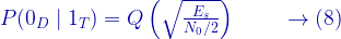
Figure 1: Simulation model for modulation and detection over flat fading channel
Simulation and performance results
In chapter 5 of the book Wireless communication systems in Matlab, the code implementation for complex baseband models for various digital modulators and demodulator are given. The computation and generation of AWGN noise is also given in the book. Using these models, we can create a unified simulation for code for simulating the performance of various modulation techniques over Rician flat-fading channel the simulation model shown in Figure 1(b).
An unified approach is employed to simulate the performance of any of the given modulation technique – MPSK, MQAM or MPAM. The simulation code (given in the book) will automatically choose the selected modulation type, performs Monte Carlo simulation, computes symbol error rates and plots them against the theoretical symbol error rate curves. The simulated performance results obtained for various modulations are shown in the Figure 2.
Figure 2: Performance of various modulations over Ricean flat fading channel
Rate this article: Note: There is a rating embedded within this post, please visit this post to rate it.
Key focus: Simulate bit error rate performance of Binary Phase Shift Keying (BPSK) modulation over AWGN channel using complex baseband equivalent model in Python & Matlab.
Why complex baseband equivalent model
The passband model and equivalent baseband model are fundamental models for simulating a communication system. In the passband model, also called as waveform simulation model, the transmitted signal, channel noise and the received signal are all represented by samples of waveforms. Since every detail of the RF carrier gets simulated, it consumes more memory and time.
In the case of discrete-time equivalent baseband model, only the value of a symbol at the symbol-sampling time instant is considered. Therefore, it consumes less memory and yields results in a very short span of time when compared to the passband models. Such models operate near zero frequency, suppressing the RF carrier and hence the number of samples required for simulation is greatly reduced. They are more suitable for performance analysis simulations. If the behavior of the system is well understood, the model can be simplified further.
In binary phase shift keying, all the information gets encoded in the phase of the carrier signal. The BPSK modulator accepts a series of information symbols drawn from the set m∈{0,1}, modulates them and transmits the modulated symbols over a channel.
The general expression for generating a M-PSK signal set is given by
Here, M denotes the modulation order and it defines the number of constellation points in the reference constellation. The value of M depends on the parameter k – the number of bits we wish to squeeze in a single M-PSK symbol. For example if we wish to squeeze in 3 bits (k=3) in one transmit symbol, then M = 2k = 23 = 8 and this results in 8-PSK configuration. M=2 gives BPSK (Binary Phase Shift Keying) configuration. The parameter A is the amplitude scaling factor, fc is the carrier frequency and g(t) is the pulse shape that satisfies orthonormal properties of basis functions.
Using trigonometric identity, equation (1) can be separated into cosine and sine basis functions as follows
Therefore, the signaling set {si,sq} or the constellation points for M-PSK modulation is given by,
For BPSK (M=2), the constellation points on the I-Q plane (Figure 1) are given by
In this simulation methodology, there is no need to simulate each and every sample of the BPSK waveform as per equation (1). Only the value of a symbol at the symbol-sampling time instant is considered. The steps for simulation of performance of BPSK over AWGN channel is as follows (Figure 2)
Generate a sequence of random bits of ones and zeros of certain length (Nsym typically set in the order of 10000)
Using the constellation points, map the bits to modulated symbols (For example, bit ‘0’ is mapped to amplitude value A, and bit ‘1’ is mapped to amplitude value -A)
Compute the total power in the sequence of modulated symbols and add noise for the given EbN0 (SNR) value (read this article on how to do this). The noise added symbols are the received symbols at the receiver.
Use thresholding technique, to detect the bits in the receiver. Based on the constellation diagram above, the detector at the receiver has to decide whether the receiver bit is above or below the threshold 0.
Compare the detected bits against the transmitted bits and compute the bit error rate (BER).
Figure 2: Simulation methodology for performance of BPSK modulation over AWGN channel
Let’s simulate the performance of BPSK over AWGN channel in Python & Matlab.
Simulation using Python
Following standalone code simulates the bit error rate performance of BPSK modulation over AWGN using Python version 3. The results are plotted in Figure 3.
Following code simulates the bit error rate performance of BPSK modulation over AWGN using basic installation of Matlab. You will need the add_awgn_noise function that was discussed in this article. The results will be same as Figure 3.
In coherent detection, the receiver derives its demodulation frequency and phase references using a carrier synchronization loop. Such synchronization circuits may introduce phase ambiguity in the detected phase, which could lead to erroneous decisions in the demodulated bits. For example, Costas loop exhibits phase ambiguity of integral multiples of radians at the lock-in points. As a consequence, the carrier recovery may lock in radians out-of-phase thereby leading to a situation where all the detected bits are completely inverted when compared to the bits during perfect carrier synchronization. Phase ambiguity can be efficiently combated by applying differential encoding at the BPSK modulator input (Figure 1) and by performing differential decoding at the output of the coherent demodulator at the receiver side (Figure 2).
In ordinary BPSK transmission, the information is encoded as absolute phases: for binary 1 and for binary 0. With differential encoding, the information is encoded as the phase difference between two successive samples. Assuming is the message bit intended for transmission, the differential encoded output is given as
The differentially encoded bits are then BPSK modulated and transmitted. On the receiver side, the BPSK sequence is coherently detected and then decoded using a differential decoder. The differential decoding is mathematically represented as
This method can deal with the phase ambiguity introduced by synchronization circuits. However, it suffers from performance penalty due to the fact that the differential decoding produces wrong bits when: a) the preceding bit is in error and the present bit is not in error , or b) when the preceding bit is not in error and the present bit is in error. After differential decoding, the average bit error rate of coherently detected BPSK over AWGN channel is given by
Figure 2: Coherent detection of differentially encoded BPSK signal
Following is the Matlab implementation of the waveform simulation model for the method discussed above. Both the differential encoding and differential decoding blocks, illustrated in Figures 1 and 2, are linear time-invariant filters. The differential encoder is realized using IIR type digital filter and the differential decoder is realized as FIR filter.
File 1: dbpsk_coherent_detection.m: Coherent detection of D-BPSK over AWGN channel
Figure 3 shows the simulated BER points together with the theoretical BER curves for differentially encoded BPSK and the conventional coherently detected BPSK system over AWGN channel.
Key focus: Derive BPSK BER (bit error rate) for optimum receiver in AWGN channel. Explained intuitively step by step.
BPSK modulation is the simplest of all the M-PSK techniques. An insight into the derivation of error rate performance of an optimum BPSK receiver is essential as it serves as a stepping stone to understand the derivation for other comparatively complex techniques like QPSK,8-PSK etc..
The ideal constellation diagram of a BPSK transmission (Figure 1) contains two constellation points located equidistant from the origin. Each constellation point is located at a distance from the origin, where Es is the BPSK symbol energy. Since the number of bits in a BPSK symbol is always one, the notations – symbol energy (Es) and bit energy (Eb) can be used interchangeably (Es=Eb).
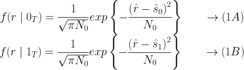
Assume that the BPSK symbols are transmitted through an AWGN channel characterized by variance = N0/2 Watts. When 0 is transmitted, the received symbol is represented by a Gaussian random variable ‘r‘ with mean=S0 = and variance =N0/2. When 1 is transmitted, the received symbol is represented by a Gaussian random variable – r with mean=S1= and variance =N0/2. Hence the conditional density function of the BPSK symbol (Figure 2) is given by,
Figure 1: BPSK – ideal constellation
Figure 2: Probability density function (PDF) for BPSK Symbols
An optimum receiver for BPSK can be implemented using a correlation receiver or a matched filter receiver (Figure 3). Both these forms of implementations contain a decision making block that decides upon the bit/symbol that was transmitted based on the observed bits/symbols at its input.
Figure 3: Optimum Receiver for BPSK
When the BPSK symbols are transmitted over an AWGN channel, the symbols appears smeared/distorted in the constellation depending on the SNR condition of the channel. A matched filter or that was previously used to construct the BPSK symbols at the transmitter. This process of projection is illustrated in Figure 4. Since the assumed channel is of Gaussian nature, the continuous density function of the projected bits will follow a Gaussian distribution. This is illustrated in Figure 5.
Figure 4: Role of correlation/Matched Filter
After the signal points are projected on the basis function axis, a decision maker/comparator acts on those projected bits and decides on the fate of those bits based on the threshold set. For a BPSK receiver, if the a-prior probabilities of transmitted 0’s and 1’s are equal (P=0.5), then the decision boundary or threshold will pass through the origin. If the apriori probabilities are not equal, then the optimum threshold boundary will shift away from the origin.
Figure 5: Distribution of received symbols
Considering a binary symmetric channel, where the apriori probabilities of 0’s and 1’s are equal, the decision threshold can be conveniently set to T=0. The comparator, decides whether the projected symbols are falling in region A or region B (see Figure 4). If the symbols fall in region A, then it will decide that 1 was transmitted. It they fall in region B, the decision will be in favor of ‘0’.
For deriving the performance of the receiver, the decision process made by the comparator is applied to the underlying distribution model (Figure 5). The symbols projected on the axis will follow a Gaussian distribution. The threshold for decision is set to T=0. A received bit is in error, if the transmitted bit is ‘0’ & the decision output is ‘1’ and if the transmitted bit is ‘1’ & the decision output is ‘0’.
This is expressed in terms of probability of error as,
Or equivalently,
By applying Bayes Theorem↗, the above equation is expressed in terms of conditional probabilities as given below,
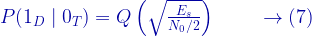
Since a-prior probabilities are equal P(0T)= P(1T) =0.5, the equation can be re-written as
Intuitively, the integrals represent the area of shaded curves as shown in Figure 6. From the previous article, we know that the area of the shaded region is given by Q function.
Figure 6a, 6b: Calculating Error Probability
Similarly,
From (4), (6), (7) and (8),
For BPSK, since Es=Eb, the probability of symbol error (Ps) and the probability of bit error (Pb) are same. Therefore, expressing the Ps and Pb in terms of Q function and also in terms of complementary error function :
Rate this article: Note: There is a rating embedded within this post, please visit this post to rate it.
The phenomenon of Rayleigh Flat fading and its simulation using Clarke’s model and Young’s model were discussed in the previous posts. The performance (Eb/N0 Vs BER) of BPSK modulation (with coherent detection) over Rayleigh Fading channel and its comparison over AWGN channel is discussed in this post.
We first investigate the non-coherent detection of BPSK over Rayleigh Fading channel and then we move on to the coherent detection. For both the cases, we consider a simple flat fading Rayleigh channel (modeled as a – single tap filter – with complex impulse response – h). The channel also adds AWGN noise to the signal samples after it suffers from Rayleigh Fading.
The received signal y can be represented as
$$ y=hx+n $$
where n is the noise contributed by AWGN which is Gaussian distributed with zero mean and unit variance and h is the Rayleigh Fading response with zero mean and unit variance. (For a simple AWGN channel without Rayleigh Fading the received signal is represented as y=x+n).
Non-Coherent Detection:
In non-coherent detection, prior knowledge of the channel impulse response (“h” in this case) is not known at the receiver. Consider the BPSK signaling scheme with ‘x=+/- a’ being transmitted over such a channel as described above. This signaling scheme fails completely (in non coherent detection scheme), even in the absence of noise, since the phase of the received signal y is uniformly distributed between 0 and 2pi regardless of whether x[m]=+a or x[m]=-a is transmitted. So the non coherent detection of the BPSK signaling is not a suitable method of detection especially in a Fading environment.
Coherent Detection:
In coherent detection, the receiver has sufficient knowledge about the channel impulse response.Techniques like pilot transmissions are used to estimate the channel impulse response at the receiver, before the actual data transmission could begin. Lets consider that the channel impulse response estimate at receiver is known and is perfect & accurate.The transmitted symbols (‘x’) can be obtained from the received signal (‘y’) by the process of equalization as given below.
$$ \hat{y}=\frac{y}{h}=\frac{hx+n}{h}=x+z $$
here z is still an AWGN noise except for the scaling factor 1/h. Now the detection of x can be performed in a manner similar to the detection in AWGN channels.
The input binary bits to the BPSK modulation system are detected as
BPSK stands for Binary Phase Shift Keying. It is a type of modulation used in digital communication systems to transmit binary data over a communication channel.
In BPSK, the carrier signal is modulated by changing its phase by 180 degrees for each binary symbol. Specifically, a binary 0 is represented by a phase shift of 180 degrees, while a binary 1 is represented by no phase shift.
BPSK is a straightforward and effective modulation method and is frequently utilized in applications where the communication channel is susceptible to noise and interference. It is also utilized in different wireless communication systems like Wi-Fi, Bluetooth, and satellite communication.
Implementation details
Binary Phase Shift Keying (BPSK) is a two phase modulation scheme, where the 0’s and 1’s in a binary message are represented by two different phase states in the carrier signal: \(\theta=0^{\circ}\) for binary 1 and \(\theta=180^{\circ}\) for binary 0.
In digital modulation techniques, a set of basis functions are chosen for a particular modulation scheme. Generally, the basis functions are orthogonal to each other. Basis functions can be derived using Gram Schmidt orthogonalizationprocedure [1]. Once the basis functions are chosen, any vector in the signal space can be represented as a linear combination of them. In BPSK, only one sinusoid is taken as the basis function. Modulation is achieved by varying the phase of the sinusoid depending on the message bits. Therefore, within a bit duration \(T_b\), the two different phase states of the carrier signal are represented as,
\begin{align*}
s_1(t) &= A_c\; cos\left(2 \pi f_c t \right), & 0 \leq t \leq T_b \quad \text{for binary 1}\\
s_0(t) &= A_c\; cos\left(2 \pi f_c t + \pi \right), & 0 \leq t \leq T_b \quad \text{for binary 0}
\end{align*}
where, \(A_c\) is the amplitude of the sinusoidal signal, \(f_c\) is the carrier frequency \(Hz\), \(t\) being the instantaneous time in seconds, \(T_b\) is the bit period in seconds. The signal \(s_0(t)\) stands for the carrier signal when information bit \(a_k=0\) was transmitted and the signal \(s_1(t)\) denotes the carrier signal when information bit \(a_k=1\) was transmitted.
The constellation diagram for BPSK (Figure 3 below) will show two constellation points, lying entirely on the x axis (inphase). It has no projection on the y axis (quadrature). This means that the BPSK modulated signal will have an in-phase component but no quadrature component. This is because it has only one basis function. It can be noted that the carrier phases are \(180^{\circ}\) apart and it has constant envelope. The carrier’s phase contains all the information that is being transmitted.
BPSK transmitter
A BPSK transmitter, shown in Figure 1, is implemented by coding the message bits using NRZ coding (\(1\) represented by positive voltage and \(0\) represented by negative voltage) and multiplying the output by a reference oscillator running at carrier frequency \(f_c\).
Figure 1: BPSK transmitter
The following function (bpsk_mod) implements a baseband BPSK transmitter according to Figure 1. The output of the function is in baseband and it can optionally be multiplied with the carrier frequency outside the function. In order to get nice continuous curves, the oversampling factor (\(L\)) in the simulation should be appropriately chosen. If a carrier signal is used, it is convenient to choose the oversampling factor as the ratio of sampling frequency (\(f_s\)) and the carrier frequency (\(f_c\)). The chosen sampling frequency must satisfy the Nyquist sampling theorem with respect to carrier frequency. For baseband waveform simulation, the oversampling factor can simply be chosen as the ratio of bit period (\(T_b\)) to the chosen sampling period (\(T_s\)), where the sampling period is sufficiently smaller than the bit period.
function [s_bb,t] = bpsk_mod(ak,L)
%Function to modulate an incoming binary stream using BPSK(baseband)
%ak - input binary data stream (0's and 1's) to modulate
%L - oversampling factor (Tb/Ts)
%s_bb - BPSK modulated signal(baseband)
%t - generated time base for the modulated signal
N = length(ak); %number of symbols
a = 2*ak-1; %BPSK modulation
ai=repmat(a,1,L).'; %bit stream at Tb baud with rect pulse shape
ai = ai(:).';%serialize
t=0:N*L-1; %time base
s_bb = ai;%BPSK modulated baseband signal
BPSK receiver
A correlation type coherent detector, shown in Figure 2, is used for receiver implementation. In coherent detection technique, the knowledge of the carrier frequency and phase must be known to the receiver. This can be achieved by using a Costas loop or a Phase Lock Loop (PLL) at the receiver. For simulation purposes, we simply assume that the carrier phase recovery was done and therefore we directly use the generated reference frequency at the receiver – \(cos( 2 \pi f_c t)\).
Figure 2: Coherent detection of BPSK (correlation type)
In the coherent receiver, the received signal is multiplied by a reference frequency signal from the carrier recovery blocks like PLL or Costas loop. Here, it is assumed that the PLL/Costas loop is present and the output is completely synchronized. The multiplied output is integrated over one bit period using an integrator. A threshold detector makes a decision on each integrated bit based on a threshold. Since, NRZ signaling format was used in the transmitter, the threshold for the detector would be set to \(0\). The function bpsk_demod, implements a baseband BPSK receiver according to Figure 2. To use this function in waveform simulation, first, the received waveform has to be downconverted to baseband, and then the function may be called.
function [ak_cap] = bpsk_demod(r_bb,L)
%Function to demodulate an BPSK(baseband) signal
%r_bb - received signal at the receiver front end (baseband)
%N - number of symbols transmitted
%L - oversampling factor (Tsym/Ts)
%ak_cap - detected binary stream
x=real(r_bb); %I arm
x = conv(x,ones(1,L));%integrate for L (Tb) duration
x = x(L:L:end);%I arm - sample at every L
ak_cap = (x > 0).'; %threshold detector
End-to-end simulation
The complete waveform simulation for the end-to-end transmission of information using BPSK modulation is given next. The simulation involves: generating random message bits, modulating them using BPSK modulation, addition of AWGN noise according to the chosen signal-to-noise ratio and demodulating the noisy signal using a coherent receiver. The topic of adding AWGN noise according to the chosen signal-to-noise ratio is discussed in section 4.1 in chapter 4. The resulting waveform plots are shown in the Figure 2.3. The performance simulation for the BPSK transmitter/receiver combination is also coded in the program shown next (see chapter 4 for more details on theoretical error rates).
The resulting performance curves will be same as the ones obtained using the complex baseband equivalent simulation technique in Figure 4.4 of chapter 4.
File 3: bpsk_wfm_sim.m: Waveform simulation for BPSK modulation and demodulation
Figure 3: (a) Baseband BPSK signal,(b) transmitted BPSK signal – with carrier, (c) constellation at transmitter and (d) received signal with AWGN noise
This website uses cookies to improve your experience while you navigate through the website. Out of these, the cookies that are categorized as necessary are stored on your browser as they are essential for the working of basic functionalities of the website. We also use third-party cookies that help us analyze and understand how you use this website. These cookies will be stored in your browser only with your consent. You also have the option to opt-out of these cookies. But opting out of some of these cookies may affect your browsing experience.
Necessary cookies are absolutely essential for the website to function properly. These cookies ensure basic functionalities and security features of the website, anonymously.
Cookie
Duration
Description
cookielawinfo-checbox-analytics
11 months
This cookie is set by GDPR Cookie Consent plugin. The cookie is used to store the user consent for the cookies in the category "Analytics".
cookielawinfo-checbox-analytics
11 months
This cookie is set by GDPR Cookie Consent plugin. The cookie is used to store the user consent for the cookies in the category "Analytics".
cookielawinfo-checbox-functional
11 months
The cookie is set by GDPR cookie consent to record the user consent for the cookies in the category "Functional".
cookielawinfo-checbox-functional
11 months
The cookie is set by GDPR cookie consent to record the user consent for the cookies in the category "Functional".
cookielawinfo-checbox-others
11 months
This cookie is set by GDPR Cookie Consent plugin. The cookie is used to store the user consent for the cookies in the category "Other.
cookielawinfo-checbox-others
11 months
This cookie is set by GDPR Cookie Consent plugin. The cookie is used to store the user consent for the cookies in the category "Other.
cookielawinfo-checkbox-necessary
11 months
This cookie is set by GDPR Cookie Consent plugin. The cookies is used to store the user consent for the cookies in the category "Necessary".
cookielawinfo-checkbox-performance
11 months
This cookie is set by GDPR Cookie Consent plugin. The cookie is used to store the user consent for the cookies in the category "Performance".
viewed_cookie_policy
11 months
The cookie is set by the GDPR Cookie Consent plugin and is used to store whether or not user has consented to the use of cookies. It does not store any personal data.
Functional cookies help to perform certain functionalities like sharing the content of the website on social media platforms, collect feedbacks, and other third-party features.
Performance cookies are used to understand and analyze the key performance indexes of the website which helps in delivering a better user experience for the visitors.
Analytical cookies are used to understand how visitors interact with the website. These cookies help provide information on metrics the number of visitors, bounce rate, traffic source, etc.


![a[k]](https://s0.wp.com/latex.php?latex=a%5Bk%5D&bg=ffffff&fg=000&s=0&c=20201002)

![b[k] = b[k-1] \oplus a[k] \;\;\;\;\;\; (modulo-2) \;\;\;\;\;\; (1)](https://s0.wp.com/latex.php?latex=b%5Bk%5D+%3D+b%5Bk-1%5D+%5Coplus+a%5Bk%5D+%5C%3B%5C%3B%5C%3B%5C%3B%5C%3B%5C%3B+%28modulo-2%29+%5C%3B%5C%3B%5C%3B%5C%3B%5C%3B%5C%3B+%281%29+&bg=ffffff&fg=000&s=2&c=20201002)

![a[k] = b[k] \oplus b[k-1] \;\;\;\;\;\; (modulo-2) \;\;\;\;\;\; (2)](https://s0.wp.com/latex.php?latex=a%5Bk%5D+%3D+b%5Bk%5D+%5Coplus+b%5Bk-1%5D%C2%A0+%5C%3B%5C%3B%5C%3B%5C%3B%5C%3B%5C%3B+%28modulo-2%29+%5C%3B%5C%3B%5C%3B%5C%3B%5C%3B%5C%3B+%282%29+&bg=ffffff&fg=000&s=2&c=20201002)


![P_b = erfc \left(\sqrt{\frac{E_b}{N_0}} \right) \left[ 1-\frac{1}{2} erfc \left( \sqrt{\frac{E_b}{N_0}} \right) \right] \;\; (3)](https://s0.wp.com/latex.php?latex=P_b+%3D+erfc+%5Cleft%28%5Csqrt%7B%5Cfrac%7BE_b%7D%7BN_0%7D%7D+%5Cright%29+%5Cleft%5B+1-%5Cfrac%7B1%7D%7B2%7D+erfc+%5Cleft%28+%5Csqrt%7B%5Cfrac%7BE_b%7D%7BN_0%7D%7D+%5Cright%29+%5Cright%5D+%5C%3B%5C%3B+%283%29+&bg=ffffff&fg=000&s=2&c=20201002)