Modified Duobinary Signaling is an extension of duobinary signaling. It has the advantage of zero PSD at low frequencies (especially at DC ) that is suitable for channels with poor DC response. It correlates two symbols that are 2T time instants apart, whereas in duobinary signaling, symbols that are 1T apart are correlated.
The general condition to achieve zero ISI is given by
As discussed in a previous article, in correlative coding , the requirement of zero ISI condition is relaxed as a controlled amount of ISI is introduced in the transmitted signal and is counteracted in the receiver side
In the case of modified duobinary signaling, the above equation is modified as
which states that the ISI is limited to two alternate samples. Here a controlled or “deterministic” amount of ISI is introduced and hence its effect can be removed upon signal detection at the receiver.
Modified Duobinary Signaling:
The following figure shows the modified duobinary signaling scheme (click to enlarge).
Modified DuoBinary Signaling
Encoding Process:
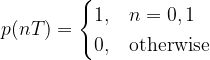
1) an = binary input bit; an ∈ {0,1}.
2) bn = NRZ polar output of Level converter in the precoder and is given by,
where ak is the precoded output (before level converter).
3) yn can be represented as
Note that the samples bn are uncorrelated ( i.e either +d for “1” or -d for “0” input). On the other-hand,the samples yn are correlated ( i.e. there are three possible values +2d,0,-2d depending on ak and ak-2). Meaning that the modified duobinary encoding correlates present sample ak and the previous input sample ak-2.
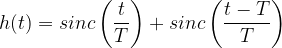
4) From the diagram,impulse response of the modified duobinary encoder is computed as
Decoding Process:
5) The receiver consists of a modified duobinary decoder and a postcoder (inverse of precoder). The decoder implements the following equation (which can be deduced from the equation given under step 3 (see above))
This equation indicates that the decoding process is prone to error propagation as the estimate of present sample relies on the estimate of previous sample. This error propagation is avoided by using a precoder before modified-duobinary encoder at the transmitter and a postcoder after the modified-duobinary decoder. The precoder ties the present sample and the sample that precedes the previous sample ( correlates these two samples) and the postcoder does the reverse process.
6) The entire process of modified-duobinary decoding and the postcoding can be combined together as one algorithm. The following decision rule is used for detecting the original modified-duobinary signal samples {an} from {yn}
The condition for zero ISI (Inter Symbol Interference) is
which states that when sampling a particular symbol (at time instant nT=0), the effect of all other symbols on the current sampled symbol is zero.
As discussed in the previous article, one of the practical ways to mitigate ISI is to use partial response signaling technique ( otherwise called as “correlative coding”). In partial response signaling, the requirement of zero ISI condition is relaxed as a controlled amount of ISI is introduced in the transmitted signal and is counteracted in the receiver side.
By relaxing the zero ISI condition, the above equation can be modified as,
which states that the ISI is limited to two adjacent samples. Here we introduce a controlled or “deterministic” amount of ISI and hence its effect can be removed upon signal detection at the receiver.
Duobinary Signaling:
The following figure shows the duobinary signaling scheme.
Figure 1: DuoBinary signaling scheme
Encoding Process:
1) an = binary input bit; an ∈ {0,1}. 2) bn = NRZ polar output of Level converter in the precoder and is given by,
3) yn can be represented as
Note that the samples bn are uncorrelated ( i.e either +d for “1” or -d for “0” input). On the other-hand, the samples yn are correlated ( i.e. there are three possible values +2d,0,-2d depending on an and an-1). Meaning that the duobinary encoding correlates present sample an and the previous input sample an-1.
4) From the diagram,impulse response of the duobinary encoder is computed as
Decoding Process:
5) The receiver consists of a duobinary decoder and a postcoder (inverse of precoder).The duobinary decoder implements the following equation (which can be deduced from the equation given under step 3 (see above))
This equation indicates that the decoding process is prone to error propagation as the estimate of present sample relies on the estimate of previous sample. This error propagation is avoided by using a precoder before duobinary encoder at the transmitter and a postcoder after the duobinary decoder. The precoder ties the present sample and previous sample ( correlates these two samples) and the postcoder does the reverse process.
6) The entire process of duobinary decoding and the postcoding can be combined together as one algorithm. The following decision rule is used for detecting the original duobinary signal samples {an} from {yn}
Note: There is a rating embedded within this post, please visit this post to rate it.
The following is a function to generate a Walsh Hadamard Matrix of given codeword size. The codeword size has to be a power of 2.
function [H]=generateHadamardMatrix(codeSize)

%[H]=generateHadamardMatrix(codeSize);
% Function to generate Walsh-Hadamard Matrix where "codeSize" is the code
% length of walsh code. The first matrix gives us two codes; 00, 01. The second
% matrix gives: 0000, 0101, 0011, 0110 and so on
% Author: Mathuranathan for https://www.gaussianwaves.com
% License: Creative Commons: Attribution-NonCommercial-ShareAlike 3.0
% Unported

%codeSize=64; %For testing only
N=2;
H=[0 0 ; 0 1];
if bitand(codeSize,codeSize-1)==0
while(N~=codeSize)
       N=N*2;
       H=repmat(H,[2,2]);
       [m,n]=size(H);

      %Invert the matrix located at the bottom right hand corner
      for i=m/2+1:m,
          for j=n/2+1:n,
                H(i,j)=~H(i,j);
         end
     end
end
else
disp('INVALID CODE SIZE:The code size must be a power of 2');
end
Example:
To Generate Walsh Codes used in IS-95 (which utilizes 64 Walsh codes of size 64 bits each, use : [H]=generateHadamardMatrix(64). This will generate 64 Walsh Codes of length 64-bits (for each code).
Test Program:
Click Here to download
Also given below is a program to test the cross-correlation and auto-correlation of Walsh code. A set of 8-Walsh codes are used for this purpose.
% Matlab Program to test Walsh Hadamard Codes and to test their orthogonality
% Plots cross-correlation and auto correlation of Walsh Hadamard Codes
% Author: Mathuranathan Viswanathan for https://www.gaussianwaves.com
% License: Creative Commons: Attribution-NonCommercial-ShareAlike 3.0
% Unported

codeSize=8;
[H]=generateHadamardMatrix(codeSize);

%-----------------------------------------------------------
%Cross-Correlation of Walsh Code 1 with rest of Walsh Codes
h = zeros(1, codeSize-1); %For dynamic Legends
s = cell(1, codeSize-1); %For dynamic Legends
for rows=2:codeSize
[crossCorrelation,lags]=crossCorr(H(1,:),H(rows,:));
h(rows-1)=plot(lags,crossCorrelation);
s{rows-1} = sprintf('Walsh Code Sequence #-%d', rows);
hold all;
end

%Dynamic Legends
% Select the plots to include in the legend
index = 1:codeSize-1;

% Create legend for the selected plots
legend(h(index),s{index});
title('Cross Correlation of Walsh Code 1 with the rest of the Walsh Codes');
ylabel('Cross Correlation');
xlabel('Lags');

%-----------------------------------------------------------
%AutoCorrelation of Walsh Code - 1
autoCorr2(H(2,:),8,2,1);
Simulation Results
From the plots below, it can be ascertained that the Walsh codes has excellent cross-correlation property and poor autocorrelation property. Excellent cross-correlation property (zero cross-correlation) implies orthogonality, which makes it suitable for CDMA applications.
Spectral leakage due to FFT is caused by: mismatch between desired tone and chosen frequency resolution, time limiting an observation. Understand the concept using hands-on examples.
Limits of frequency domain studies
Frequency Transform is used to study a signal’s frequency domain characteristics. When using FFT to study the frequency domain characteristics of a signal, there are two limits : 1) The detect-ability of a small signal in the presence of a larger one; 2) frequency resolution – which distinguishes two different frequencies.
In practice, the measured signals are limited in time and the FFT calculates the frequency transform over a certain number of discrete frequencies called bins.
Spectral Leakage:
In reality, signals are of time-limited nature and nothing can be known about the signal beyond the measured interval. For example, if the measurement of a never ending continuous train of sinusoidal wave is of interest, at some point of time we need to terminate our observation to do further analysis. The limit on the time is also posed by limitations of the measurement system itself (example: buffer size), besides other factors.
It is often said that the FFT implicitly assumes that the signal essentially repeats itself after the measured interval and hence the FFT assumes the signal to be continuous (conceptually, juxtapose the measured signal repetitively). This lead to glitches in the assumed signal (see Figure 1). When the measurement time is purposefully made to be a non-integral multiple of the actual signal rate, these sharp discontinuities will spread out in the frequency domain leading to spectral leakage. This explanation for spectral leakage need to be carefully investigated.
Figure 1:Impact of observation interval on FFT
Experiment 1: Effect of FFT length and frequency resolution
Consider a pure sinusoidal signal of frequency \(f_x = 10 \;Hz\) and to represent in computer memory, the signal is observed for 1 second and sampled at frequency \(F_s=100 \; Hz\). Now, there will be 100 samples in the buffer and the buffer will contain integral number of waveform cycles (10 cycles in this case). The signal samples are analyzed using N-point DFT. Two cases are considered here for investigation : 1) The FFT size \(N\) is same as the length of the signal samples, i.e, N=100 and 2) FFT size set to next power of 2 that fits the signal samples i.e, N=128. The result are plotted next.
Fx=10; %Frequency of the sinusoid
Fs=100; %Sampling Frequency
observationTime = 1; %observation time in seconds
t=0:1/Fs:observationTime-1/Fs; %time base
x=sin(2*pi*Fx*t);%sampled sine wave

N=100; %DFT length same as signal length
X1 = 1/N*fftshift(fft(x,N));%N-point complex DFT of x
f1=(-N/2:1:N/2-1)*Fs/N; %frequencies on x-axis, Fs/N is the frequency resolution

N=128; %DFT length
X2 = 1/N*fftshift(fft(x,N));%N-point complex DFT of x
f2=(-N/2:1:N/2-1)*Fs/N; %frequencies on x-axis, Fs/N is the frequency resolution

figure;
subplot(3,1,1);stem(x,'r')
title('Time domain');xlabel('Sample index (n)');ylabel('x[n]');
subplot(3,1,2);stem(f1,abs(X1)); %magnitudes vs frequencies
xlim([-16,16]);title(['FFT, N=100, \Delta f=',num2str(Fs/100)]);xlabel('f (Hz)'); ylabel('|X(k)|');
subplot(3,1,3);stem(f2,abs(X2)); %magnitudes vs frequencies
xlim([-16,16]);title(['FFT, N=128, \Delta f=',num2str(Fs/128)]);xlabel('f (Hz)'); ylabel('|X(k)|');
Figure 2: Effect of FFT length and frequency resolution
One might wonder, even though the buffered samples contain integral number of waveform cycles, why the frequency spectrum registered a distinct spike at \(10 \; Hz\) when \(N=100\) and not when \(N=128\). This is due to the different frequency resolution, the measure of ability to resolve two different adjacent frequencies
For case 1, the frequency resolution is \(\Delta f = f_s/N = 100/10 = 1 Hz\). This means that the frequency bins are spaced 1 Hz apart and that is why it is able to hit the bull’s eye at 10 Hz peak.
For case 2, the frequency resolution is \(\Delta f = f_s/128 = 100/128 = 0.7813 Hz\). With this frequency resolution, the x-axis of the frequency plot cannot have exact value of 10 Hz. Instead, the nearest adjacent frequency bins are 9.375 Hz and 10.1563 Hz respectively. Therefore, the frequency spectrum cannot represent 10 Hz and the energy of the signal gets leaked to adjacent bins, leading to spectral leakage.
Experiment 2: Effect of time-limited observation
In the previous experiment, the signal wave observed for 1 second duration and that fetched whole 10 cycles in the signal buffer. Now, reduce the observation time to 0.91 second and re-run the same code, results below. In this case, the signal buffer will have 9.1 cycles of the sinewave, which is not a whole number. For case 1, the frequency resolution is 1 Hz and the FFT plot has registered a distinct peak at 10 Hz. Careful investigation of the plot will reveal very low spectral leakage even in case 1 (observe the non-zero amplitude values for the rest of the bins). This is primarily due to the change in the observation interval leading to non-integral number of cycles within the observed window. The spectral leakage in case 2, when N=128, is predominantly due to mismatch in the frequency resolution.
Figure 3: Effect of limited time observation on spectral leakage in time domain
From these two experiments, we can say that 1) The mismatch between the tone of the signal and the chosen frequency resolution (result of sampling frequency and the FFT length) leads to spectral leakage (experiment 1). 2) Time-limiting an observation (at inappropriate times), may lead to spectral leakage (experiment 2). 3) Hence, the spectral leakage from a larger signal component, if present, may significantly overshadow other smaller signals making them difficult to identify or detect.
Rate this article: Note: There is a rating embedded within this post, please visit this post to rate it.
The moving average filter is a simple Low Pass FIR (Finite Impulse Response) filter commonly used for smoothing an array of sampled data/signal. It takes samples of input at a time and takes the average of those -samples and produces a single output point. It is a very simple LPF (Low Pass Filter) structure that comes handy for scientists and engineers to filter unwanted noisy component from the intended data.
As the filter length increases (the parameter ) the smoothness of the output increases, whereas the sharp transitions in the data are made increasingly blunt. This implies that this filter has excellent time domain response but a poor frequency response.
The MA filter performs three important functions:
1) It takes input points, computes the average of those -points and produces a single output point 2) Due to the computation/calculations involved, the filter introduces a definite amount of delay 3) The filter acts as a Low Pass Filter (with poor frequency domain response and a good time domain response).
Implementation
The difference equation for a -point discrete-time moving average filter with input represented by the vector and the averaged output vector , is
For example, a -point Moving Average FIR filter takes the current and previous four samples of input and calculates the average. This operation is represented as shown in the Figure 1 with the following difference equation for the input output relationship in discrete-time.
Figure 1: Discrete-time 5-point Moving Average FIR filter
The unit delay shown in Figure 1 is realized by either of the two options:
Representing the input samples as an array in the computer memory and processing them
Using D-Flip flop shift registers for digital hardware implementation. If each discrete value of the input is represented as a -bit signal line from ADC (analog to digital converter), then we would require 4 sets of 12-Flip flops to implement the -point moving average filter shown in Figure 1.
Z-Transform and Transfer function
In signal processing, delaying a signal by sample period (unit delay) is equivalent to multiplying the Z-transform by . By applying this idea, we can find the Z-transform of the -point moving average filter in equation (2) as
The transfer function describes the input-output relationship of the system and for the -point Moving Average filter, the transfer function is given by
where, and are the filter coefficients and the order of the filter is the maximum of and
For implementing equation (6) using the filter function, the Matlab function is called as
B = [b_0, b_1, b_2, ..., b_n] %numerator coefficients
A = [a_0, a_1, a_2, ..., a_m] %denominator coefficients
y = filter(B,A,x) %filter input x and get result in y
We can note from the difference equation and transfer function of the -point moving average filter, that following values for the numerator coefficients and denominator coefficients .
Therefore, the -point moving average filter can be coded as
B = [0.2, 0.2, 0.2, 0.2, 0.2] %numerator coefficients
A = [1] %denominator coefficients
y = filter(B,A,x) %filter input x and get result in y
The numerator coefficients for the moving average filter can be conveniently expressed in short notion as shown below
 L = 5
B = ones(1,L)/L %numerator coefficients
A = [1] %denominator coefficients
x = rand(1,10) %random samples for x
y = filter(B,A,x) %filter input x and get result in y
When using conv function to implement the moving average filter, the following code can be used
L = 5;
x = rand(1,10) %random samples for x;
y = conv(x,ones(1,L)/L)
There exists a difference between using conv function and filter function for implementing an FIR filter. The conv function gives the result of complete convolution and the length of the result is length(x)+ L -1. Whereas, the filter function gives the output that is of same length as that of the input .
In python, the filtering operation can be performed using the lfilter and convolve functions available in the scipy signal processing package. The equivalent python code is shown below.
import numpy as np
from scipy import signal
L=5 #L-point filter
b = (np.ones(L))/L #numerator co-effs of filter transfer function
a = np.ones(1)  #denominator co-effs of filter transfer function
x = np.random.randn(10) #10 random samples for x
y = signal.convolve(x,b) #filter output using convolution

y = signal.lfilter(b,a,x) #filter output using lfilter function
Pole-zero plot and frequency response
A pole-zero plot for a filter transfer function , displays the pole and zero locations in the z-plane. In the pole-zero plot, the zeros occur at locations (frequencies) where and the poles occur at locations (frequencies) where . Equivalently, zeros occurs at frequencies for which the numerator of the transfer function in equation 6 becomes zero and the poles occurs at frequencies for which the denominator of the transfer function becomes zero.
In a pole-zero plot, the locations of the poles are usually marked by cross () and the zeros are marked as circles (). The poles and zeros of a transfer function effectively define the system response and determines the stability and performance of the filtering system.
In Matlab, the pole-zero plot and the frequency response of the -point moving average can be obtained as follows.
L=11
zplane([ones(1,L)]/L,1); %pole-zero plot
w = -pi:(pi/100):pi; %to plot frequency response
freqz([ones(1,L)]/L,1,w); %plot magnitude and phase response
Figure 2: Pole-Zero plot for L=11-point Moving Average filter
Figure 3: Magnitude and phase response of L=11-point Moving Average filter
The magnitude and phase frequency responses can be coded in Python as follows
import numpy as np
from scipy import signal
import matplotlib.pyplot as plt

L=11 #L-point filter
b = (np.ones(L))/L #numerator co-effs of filter transfer function
a = np.ones(1)  #denominator co-effs of filter transfer function

w, h = signal.freqz(b,a)
plt.subplot(2, 1, 1)
plt.plot(w, 20 * np.log10(abs(h)))
plt.ylabel('Magnitude [dB]')
plt.xlabel('Frequency [rad/sample]')

plt.subplot(2, 1, 2)
angles = np.unwrap(np.angle(h))
plt.plot(w, angles)
plt.ylabel('Angle (radians)')
plt.xlabel('Frequency [rad/sample]')
plt.show()
Figure 4: Impulse response, Pole-zero plot, magnitude and phase response of L=11 moving average filter
Case study:
Following figures depict the time domain & frequency domain responses of a -point Moving Average filter. A noisy square wave signal is driven through the filter and the time domain response is obtained.
Figure 5: Processing a signal through Moving average filter of various lengths
On the first plot, we have the noisy square wave signal that is going into the moving average filter. The input is noisy and our objective is to reduce the noise as much as possible. The next figure is the output response of a 3-point Moving Average filter. It can be deduced from the figure that the 3-point Moving Average filter has not done much in filtering out the noise. We increase the filter taps to 10-points and we can see that the noise in the output has reduced a lot, which is depicted in next figure.
With L=51 tap filter, though the noise is almost zero, the transitions are blunted out drastically (observe the slope on the either side of the signal and compare them with the ideal brick wall transitions in the input signal).
From the frequency response of lower order filters (L=3, L=10), it can be asserted that the roll-off is very slow and the stop band attenuation is not good. Given this stop band attenuation, clearly, the moving average filter cannot separate one band of frequencies from another. As we increase the filter order to 51, the transitions are not preserved in time domain. Good performance in the time domain results in poor performance in the frequency domain, and vice versa. Compromise need for optimal filter design.
Rate this article: Note: There is a rating embedded within this post, please visit this post to rate it.
Note: There is a rating embedded within this post, please visit this post to rate it.
Random Interleaver:
The Random Interleaver rearranges the elements of its input vector using a random permutation. The incoming data is rearranged using a series of generated permuter indices. A permuter is essentially a device that generates pseudo-random permutation of given memory addresses. The data is arranged according to the pseudo-random order of memory addresses.
The de-interleaver must know the permuter-indices exactly in the same order as that of the interleaver. The de-interleaver arranges the interleaved data back to the original state by knowing the permuter-indices.
Random Interleaver
The interleaver depth (D) (Not sure what this term means ? – check out this article – click here) is essentially the number of memory addresses taken for permutation at a time. If the number of memory addresses taken for permutation increases, the interleaver depth increases.
In the Matlab simulation that is given below, an interleaver depth of 15 is used for illustration. This means that 15 letters are taken at a time and are permuted (rearranged randomly). This process is repeated consecutively for the next block of 15 letters.
As you may observe from the simulation that increasing the interleaver depth will increase the degree of randomness in the interleaved data and will decrease the maximum burst length after the de-interleaver operation.
Matlab Code:
A sample Matlab code that simulates the above mentioned random interleaver is given below. The input data is a repeatitive stream of following symbols – “THE_QUICK_BROWN_FOX_JUMPS_OVER_THE_LAZY_DOG_“. This code simulates only the interleaving/de-interleaving part.The burst errors produced by channel are denoted by ‘*‘.
%Demonstration of PseudoRandom Interleaver/Deinterleaver
%Author : Mathuranathan for https://www.gaussianwaves.com
%License - Creative Commons - cc-by-nc-sa 3.0

clc;
clear;
%____________________________________________
%Input Parameters
%____________________________________________
D=15; %Interleaver Depth. More the value of D more is the randomness
n=5; %Number of Data blocks that you want to send.
data='THE_QUICK_BROWN_FOX_JUMPS_OVER_THE_LAZY_DOG_'; % A constant pattern used as a data
%____________________________________________
%Make the length of the data to be a multiple of D. This is for
%demonstration only.Otherwise the empty spaces has to be zero filled.
data=repmat(data,1,n); %send n blocks of specified data pattern
if mod(length(data),D) ~=0
    data=[data data(1:(D*(fix(length(data)/D+1))-length(data)))];
end

%We are sending D blocks of similar data
%intlvrInput=repmat(data(1:n),[1 D]);
%fprintf('Input Data to the Interleaver -> \n');
%disp(char(intlvrInput));
%disp('____________________________________________________________________________');

%INTERLEAVER
%Writing into the interleaver row-by-row
permuterIndex=randperm(D);
intrlvrOutput=[];
index=1;

for i=1:fix(length(data)/D)
    intrlvrOutput=[intrlvrOutput data(permuterIndex+(i-1)*D)];
end

for i=1:mod(length(data),D)
    intrlvrOutput=[intrlvrOutput data(permuterIndex(i)+fix(length(data)/D)*D)];
end

uncorruptedIntrlvrOutput=intrlvrOutput;

%Corrupting the interleaver output by inserting 10 '*'
intrlvrOutput(1,25:34)=zeros(1,10)+42;

%DEINTERLEAVER
deintrlvrOutput=[];

for i=1:fix(length(intrlvrOutput)/D)
    deintrlvrOutput(permuterIndex+(i-1)*D)=intrlvrOutput((i-1)*D+1:i*D);
end

for i=1:mod(length(intrlvrOutput),D)
    deintrlvrOutput((fix(length(intrlvrOutput)/D))*permuterIndex+i)=intrlvrOutput((i+1):(i+1)*D);
end

deintrlvrOutput=char(deintrlvrOutput);
disp('Given Data -->');
disp(data);
disp(' ')
disp('Permuter Index-->')
disp(permuterIndex);
disp(' ')
disp('PseudoRandom Interleaver Output -->');
disp(uncorruptedIntrlvrOutput);
disp(' ')
disp('Interleaver Output after being corrupted by 10 symbols of burst error - marked by ''*''->');
disp(char(intrlvrOutput));
disp(' ')
disp('PseudoRandom Deinterleaver Output -->');
disp(deintrlvrOutput);
Simulation Result:
Given Data –>
THE_QUICK_BROWN_FOX_JUMPS_OVER_THE_LAZY_DOG_THE_QUICK_BROWN_FOX
_JUMPS_OVER_THE_LAZY_DOG_THE_QUICK_BROWN_FOX_JUMPS_OVER_THE_LAZY
_DOG_THE_QUICK_BROWN_FOX_JUMPS_OVER_THE_LAZY_DOG_THE_QUICK_BROWN
_FOX_JUMPS_OVER_THE_LAZY_DOG_THE_Q
Interleaver Output after being corrupted by 10 symbols of burst error – marked by ‘*‘->
NTBKIRQUO_H_ECWR__PUO_JV**********AO_LGET_HZ__HR_COUIWQEB_KN_FOS
MVJUE_O_XPRHTO_ZGLA__HDEYTFEOBKWICNU_RQ__TOV_PEUMRJXO_S_EHGDY
_AZTLEO__HO_WR_NCK_IQOUBFHXEOSRMP_U_VJ_T_E_O_TZYHA_GLDEXQNOB_K
_FCUWIROE_RV__PSTMJEUOHQ_TGDHY_EZL_AO_
As we can see from the above simulation that, even though the channel introduces 10 symbols of consecutive burst error, the interleaver/deinterleaver operation has effectively distributed the errors and reduced the maximum burst length to 3 symbols.
Quadrature Phase Shift Keying (QPSK) is a form of phase modulation technique, in which two information bits (combined as one symbol) are modulated at once, selecting one of the four possible carrier phase shift states.
Figure 1: Waveform simulation model for QPSK modulation
The QPSK signal within a symbol duration \(T_{sym}\) is defined as
\[s(t) = A \cdot cos \left[2 \pi f_c t + \theta_n \right], \quad \quad 0 \leq t \leq T_{sym},\; n=1,2,3,4 \quad \quad (1) \]
Therefore, the four possible initial signal phases are \(\pi/4, 3 \pi/4, 5 \pi/4\) and \(7 \pi/4\) radians. Equation (1) can be re-written as
\[\begin{align} s(t) &= A \cdot cos \theta_n \cdot cos \left( 2 \pi f_c t\right) – A \cdot sin \theta_n \cdot sin \left( 2 \pi f_c t\right) \\ &= s_{ni} \phi_i(t) + s_{nq} \phi_q(t) \quad\quad \quad \quad \quad\quad \quad \quad \quad\quad \quad \quad \quad\quad \quad \quad (3) \end{align} \]
The above expression indicates the use of two orthonormal basis functions: \( \left\langle \phi_i(t),\phi_q(t)\right\rangle\) together with the inphase and quadrature signaling points: \( \left\langle s_{ni}, s_{nq}\right\rangle\). Therefore, on a two dimensional co-ordinate system with the axes set to \( \phi_i(t)\) and \(\phi_q(t)\), the QPSK signal is represented by four constellation points dictated by the vectors \(\left\langle s_{ni}, s_{nq}\right\rangle\) with \( n=1,2,3,4\).
The QPSK transmitter, shown in Figure 1, is implemented as a matlab function qpsk_mod. In this implementation, a splitter separates the odd and even bits from the generated information bits. Each stream of odd bits (quadrature arm) and even bits (in-phase arm) are converted to NRZ format in a parallel manner.
function [s,t,I,Q] = qpsk_mod(a,fc,OF)
%Modulate an incoming binary stream using conventional QPSK
%a - input binary data stream (0's and 1's) to modulate
%fc - carrier frequency in Hertz
%OF - oversampling factor (multiples of fc) - at least 4 is better
%s - QPSK modulated signal with carrier
%t - time base for the carrier modulated signal
%I - baseband I channel waveform (no carrier)
%Q - baseband Q channel waveform (no carrier)
L = 2*OF;%samples in each symbol (QPSK has 2 bits in each symbol)
ak = 2*a-1; %NRZ encoding 0-> -1, 1->+1
I = ak(1:2:end);Q = ak(2:2:end);%even and odd bit streams
I=repmat(I,1,L).'; Q=repmat(Q,1,L).';%even/odd streams at 1/2Tb baud
I = I(:).'; Q = Q(:).'; %serialize
fs = OF*fc; %sampling frequency
t=0:1/fs:(length(I)-1)/fs; %time base
iChannel = I.*cos(2*pi*fc*t);qChannel = -Q.*sin(2*pi*fc*t);
s = iChannel + qChannel; %QPSK modulated baseband signal
The timing diagram for BPSK and QPSK modulation is shown in Figure 2. For BPSK modulation the symbol duration for each bit is same as bit duration, but for QPSK the symbol duration is twice the bit duration: \(T_{sym}=2T_b\). Therefore, if the QPSK symbols were transmitted at same rate as BPSK, it is clear that QPSK sends twice as much data as BPSK does. After oversampling and pulse shaping, it is intuitively clear that the signal on the I-arm and Q-arm are BPSK signals with symbol duration \(2T_b\). The signal on the in-phase arm is then multiplied by \(cos (2 \pi f_c t)\) and the signal on the quadrature arm is multiplied by \(-sin (2 \pi f_c t)\). QPSK modulated signal is obtained by adding the signal from both in-phase and quadrature arms.
Note: The oversampling rate for the simulation is chosen as \(L=2 f_s/f_c\), where \(f_c\) is the given carrier frequency and \(f_s\) is the sampling frequency satisfying Nyquist sampling theorem with respect to the carrier frequency (\(f_s \geq f_c\)). This configuration gives integral number of carrier cycles for one symbol duration.
Figure 2: Timing diagram for BPSK and QPSK modulations
The receiver
Due to its special relationship with BPSK, the QPSK receiver takes the simplest form as shown in Figure 3. In this implementation, the I-channel and Q-channel signals are individually demodulated in the same way as that of BPSK demodulation. After demodulation, the I-channel bits and Q-channel sequences are combined into a single sequence. The function qpsk_demod implements a QPSK demodulator as per Figure 3.
Read more about QPSK, implementation of their modulator and demodulator, performance simulation in these books:
Figure 3: Waveform simulation model for QPSK demodulation
Performance simulation over AWGN
The complete waveform simulation for the aforementioned QPSK modulation and demodulation is given next. The simulation involves, generating random message bits, modulating them using QPSK modulation, addition of AWGN channel noise corresponding to the given signal-to-noise ratio and demodulating the noisy signal using a coherent QPSK receiver. The waveforms at the various stages of the modulator are shown in the Figure 4.
Figure 4: Simulated QPSK waveforms at the transmitter side
The performance simulation for the QPSK transmitter-receiver combination was also coded in the code given above and the resulting bit-error rate performance curve will be same as that of conventional BPSK. A QPSK signal essentially combines two orthogonally modulated BPSK signals. Therefore, the resulting performance curves for QPSK – \(E_b/N_0\) Vs. bits-in-error – will be same as that of conventional BPSK.
QPSK variants
QPSK modulation has several variants, three such flavors among them are: Offset QPSK, π/4-QPSK and π/4-DQPSK.
Offset-QPSK
Offset-QPSK is essentially same as QPSK, except that the orthogonal carrier signals on the I-channel and the Q-channel are staggered (one of them is delayed in time). In OQPSK, the orthogonal components cannot change states at the same time, this is because the components change state only at the middle of the symbol periods (due to the half symbol offset in the Q-channel). This eliminates 180° phase shifts all together and the phase changes are limited to 0° or 90° every bit period.
Elimination of 180° phase shifts in OQPSK offers many advantages over QPSK. Unlike QPSK, the spectrum of OQPSK remains unchanged when band-limited [1]. Additionally, OQPSK performs better than QPSK when subjected to phase jitters [2]. Further improvements to OQPSK can be obtained if the phase transitions are avoided altogether – as evident from continuous modulation schemes like Minimum Shift Keying (MSK) technique.
π/4-QPSK and π/4-DQPSK
In π/4-QPSK, the signaling points of the modulated signals are chosen from two QPSK constellations that are just shifted π/4 radians (45°) with respect to each other. Switching between the two constellations every successive bit ensures that the phase changes are confined to odd multiples of 45°. Therefore, phase transitions of 90° and 180° are eliminated.
π/4-QPSK preserves the constant envelope property better than QPSK and OQPSK. Unlike QPSK and OQPSK schemes, π/4-QPSK can be differentially encoded, therefore enabling the use of both coherent and non-coherent demodulation techniques. Choice of non-coherent demodulation results in simpler receiver design. Differentially encoded π/4-QPSK is referred as π/4-DQPSK.
Read more about QPSK and its variants, implementation of their modulator and demodulator, performance simulation in these books:
Key focus: Compare Performance and spectral efficiency of bandwidth-efficient digital modulation techniques (BPSK,QPSK and QAM) on their theoretical BER over AWGN.
Let’s take up some bandwidth-efficient linear digital modulation techniques (BPSK,QPSK and QAM) and compare its performance based on their theoretical BER over AWGN. (Readers are encouraged to read previous article on Shannon’s theorem and channel capacity).
Table 1 summarizes the theoretical BER (given SNR per bit ration – Eb/N0) for various linear modulations. Note that the Eb/N0 values used in that table are in linear scale [to convert Eb/N0 in dB to linear scale – use Eb/N0(linear) = 10^(Eb/N0(dB)/10) ]. A small script written in Matlab (given below) gives the following output.
Figure 1: Eb/N0 Vs. BER for various digital modulations over AWGN channel
Table 1: Theoretical BER over AWGN for various linear digital modulation techniques
The following table is obtained by extracting the values of Eb/N0 to achieve BER=10-6 from Figure-1. (Table data sorted with increasing values of Eb/N0).
Table 2: Capacity of various modulations their efficiency and channel bandwidth
where,
is the bandwidth efficiency for linear modulation with M point constellation, meaning that ηBbits can be stuffed in one symbol with Rb bits/sec data rate for a given minimum bandwidth.
is the minimum bandwidth needed for information rate of Rb bits/second. If a pulse shaping technique like raised cosine pulse [with roll off factor (a)] is used then Bmin becomes
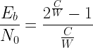
Next the data in table 2 is plotted with Eb/N0 on the x-axis and ηon the y-axis (see figure 2) along with the well known Shannon’s Capacity equation over AWGN given by,
which can be represented as (refer [1])
Figure 2: Spectral efficiency vs Eb/N0 for various modulations at Pb=10-6
Rate this article: Note: There is a rating embedded within this post, please visit this post to rate it.
Matlab Code
EbN0dB=-4:1:24;
EbN0lin=10.^(EbN0dB/10);
colors={'b-*','g-o','r-h','c-s','m-d','y-*','k-p','b-->','g:<','r-.d'};
index=1;

%BPSK
BPSK = 0.5*erfc(sqrt(EbN0lin));
plotHandle=plot(EbN0dB,log10(BPSK),char(colors(index)));
set(plotHandle,'LineWidth',1.5);
hold on;

index=index+1;

%M-PSK
m=2:1:5;
M=2.^m;
for i=M,
    k=log2(i);
    berErr = 1/k*erfc(sqrt(EbN0lin*k)*sin(pi/i));
    plotHandle=plot(EbN0dB,log10(berErr),char(colors(index)));
    set(plotHandle,'LineWidth',1.5);
    index=index+1;
end

%Binary DPSK
Pb = 0.5*exp(-EbN0lin);
plotHandle = plot(EbN0dB,log10(Pb),char(colors(index)));
set(plotHandle,'LineWidth',1.5);
index=index+1;

%Differential QPSK
a=sqrt(2*EbN0lin*(1-sqrt(1/2)));
b=sqrt(2*EbN0lin*(1+sqrt(1/2)));
Pb = marcumq(a,b,1)-1/2.*besseli(0,a.*b).*exp(-1/2*(a.^2+b.^2));
plotHandle = plot(EbN0dB,log10(Pb),char(colors(index)));
set(plotHandle,'LineWidth',1.5);
index=index+1;

%M-QAM
m=2:2:6;
M=2.^m;

for i=M,
    k=log2(i);
    berErr = 2/k*(1-1/sqrt(i))*erfc(sqrt(3*EbN0lin*k/(2*(i-1))));
    plotHandle=plot(EbN0dB,log10(berErr),char(colors(index)));
    set(plotHandle,'LineWidth',1.5);
    index=index+1;
end

legend('BPSK','QPSK','8-PSK','16-PSK','32-PSK','D-BPSK','D-QPSK','4-QAM','16-QAM','64-QAM');
axis([-4 24 -8 0]);
set(gca,'XTick',-4:2:24); %re-name axis accordingly
ylabel('Probability of BER Error - log10(Pb)');
xlabel('Eb/N0 (dB)');
title('Probability of BER Error log10(Pb) Vs Eb/N0');
grid on;
BPSK stands for Binary Phase Shift Keying. It is a type of modulation used in digital communication systems to transmit binary data over a communication channel.
In BPSK, the carrier signal is modulated by changing its phase by 180 degrees for each binary symbol. Specifically, a binary 0 is represented by a phase shift of 180 degrees, while a binary 1 is represented by no phase shift.
BPSK is a straightforward and effective modulation method and is frequently utilized in applications where the communication channel is susceptible to noise and interference. It is also utilized in different wireless communication systems like Wi-Fi, Bluetooth, and satellite communication.
Implementation details
Binary Phase Shift Keying (BPSK) is a two phase modulation scheme, where the 0’s and 1’s in a binary message are represented by two different phase states in the carrier signal: \(\theta=0^{\circ}\) for binary 1 and \(\theta=180^{\circ}\) for binary 0.
In digital modulation techniques, a set of basis functions are chosen for a particular modulation scheme. Generally, the basis functions are orthogonal to each other. Basis functions can be derived using Gram Schmidt orthogonalizationprocedure [1]. Once the basis functions are chosen, any vector in the signal space can be represented as a linear combination of them. In BPSK, only one sinusoid is taken as the basis function. Modulation is achieved by varying the phase of the sinusoid depending on the message bits. Therefore, within a bit duration \(T_b\), the two different phase states of the carrier signal are represented as,
\begin{align*}
s_1(t) &= A_c\; cos\left(2 \pi f_c t \right), & 0 \leq t \leq T_b \quad \text{for binary 1}\\
s_0(t) &= A_c\; cos\left(2 \pi f_c t + \pi \right), & 0 \leq t \leq T_b \quad \text{for binary 0}
\end{align*}
where, \(A_c\) is the amplitude of the sinusoidal signal, \(f_c\) is the carrier frequency \(Hz\), \(t\) being the instantaneous time in seconds, \(T_b\) is the bit period in seconds. The signal \(s_0(t)\) stands for the carrier signal when information bit \(a_k=0\) was transmitted and the signal \(s_1(t)\) denotes the carrier signal when information bit \(a_k=1\) was transmitted.
The constellation diagram for BPSK (Figure 3 below) will show two constellation points, lying entirely on the x axis (inphase). It has no projection on the y axis (quadrature). This means that the BPSK modulated signal will have an in-phase component but no quadrature component. This is because it has only one basis function. It can be noted that the carrier phases are \(180^{\circ}\) apart and it has constant envelope. The carrier’s phase contains all the information that is being transmitted.
BPSK transmitter
A BPSK transmitter, shown in Figure 1, is implemented by coding the message bits using NRZ coding (\(1\) represented by positive voltage and \(0\) represented by negative voltage) and multiplying the output by a reference oscillator running at carrier frequency \(f_c\).
Figure 1: BPSK transmitter
The following function (bpsk_mod) implements a baseband BPSK transmitter according to Figure 1. The output of the function is in baseband and it can optionally be multiplied with the carrier frequency outside the function. In order to get nice continuous curves, the oversampling factor (\(L\)) in the simulation should be appropriately chosen. If a carrier signal is used, it is convenient to choose the oversampling factor as the ratio of sampling frequency (\(f_s\)) and the carrier frequency (\(f_c\)). The chosen sampling frequency must satisfy the Nyquist sampling theorem with respect to carrier frequency. For baseband waveform simulation, the oversampling factor can simply be chosen as the ratio of bit period (\(T_b\)) to the chosen sampling period (\(T_s\)), where the sampling period is sufficiently smaller than the bit period.
function [s_bb,t] = bpsk_mod(ak,L)
%Function to modulate an incoming binary stream using BPSK(baseband)
%ak - input binary data stream (0's and 1's) to modulate
%L - oversampling factor (Tb/Ts)
%s_bb - BPSK modulated signal(baseband)
%t - generated time base for the modulated signal
N = length(ak); %number of symbols
a = 2*ak-1; %BPSK modulation
ai=repmat(a,1,L).'; %bit stream at Tb baud with rect pulse shape
ai = ai(:).';%serialize
t=0:N*L-1; %time base
s_bb = ai;%BPSK modulated baseband signal
BPSK receiver
A correlation type coherent detector, shown in Figure 2, is used for receiver implementation. In coherent detection technique, the knowledge of the carrier frequency and phase must be known to the receiver. This can be achieved by using a Costas loop or a Phase Lock Loop (PLL) at the receiver. For simulation purposes, we simply assume that the carrier phase recovery was done and therefore we directly use the generated reference frequency at the receiver – \(cos( 2 \pi f_c t)\).
Figure 2: Coherent detection of BPSK (correlation type)
In the coherent receiver, the received signal is multiplied by a reference frequency signal from the carrier recovery blocks like PLL or Costas loop. Here, it is assumed that the PLL/Costas loop is present and the output is completely synchronized. The multiplied output is integrated over one bit period using an integrator. A threshold detector makes a decision on each integrated bit based on a threshold. Since, NRZ signaling format was used in the transmitter, the threshold for the detector would be set to \(0\). The function bpsk_demod, implements a baseband BPSK receiver according to Figure 2. To use this function in waveform simulation, first, the received waveform has to be downconverted to baseband, and then the function may be called.
function [ak_cap] = bpsk_demod(r_bb,L)
%Function to demodulate an BPSK(baseband) signal
%r_bb - received signal at the receiver front end (baseband)
%N - number of symbols transmitted
%L - oversampling factor (Tsym/Ts)
%ak_cap - detected binary stream
x=real(r_bb); %I arm
x = conv(x,ones(1,L));%integrate for L (Tb) duration
x = x(L:L:end);%I arm - sample at every L
ak_cap = (x > 0).'; %threshold detector
End-to-end simulation
The complete waveform simulation for the end-to-end transmission of information using BPSK modulation is given next. The simulation involves: generating random message bits, modulating them using BPSK modulation, addition of AWGN noise according to the chosen signal-to-noise ratio and demodulating the noisy signal using a coherent receiver. The topic of adding AWGN noise according to the chosen signal-to-noise ratio is discussed in section 4.1 in chapter 4. The resulting waveform plots are shown in the Figure 2.3. The performance simulation for the BPSK transmitter/receiver combination is also coded in the program shown next (see chapter 4 for more details on theoretical error rates).
The resulting performance curves will be same as the ones obtained using the complex baseband equivalent simulation technique in Figure 4.4 of chapter 4.
File 3: bpsk_wfm_sim.m: Waveform simulation for BPSK modulation and demodulation
Figure 3: (a) Baseband BPSK signal,(b) transmitted BPSK signal – with carrier, (c) constellation at transmitter and (d) received signal with AWGN noise
Gibbs phenomenon is a phenomenon that occurs in signal processing and Fourier analysis when approximating a discontinuous function using a series of Fourier coefficients. Specifically, it is the observation that the overshoots near the discontinuities of the approximated function do not decrease with increasing numbers of Fourier coefficients used in the approximation.
In other words, when a discontinuous function is approximated by its Fourier series, the resulting series will exhibit oscillations near the discontinuities that do not diminish as more terms are added to the series. This can lead to a “ringing” effect in the signal, where there are spurious oscillations near the discontinuity that can persist even when the number of Fourier coefficients used in the approximation is increased.
The Gibbs phenomenon is named after American physicist Josiah Willard Gibbs, who first described it in 1899. It is a fundamental limitation of the Fourier series approximation and can occur in many other areas of signal processing and analysis as well.
Gibbs phenomenon
Fourier transform represents signals in frequency domain as summation of unique combination of sinusoidal waves. Fourier transforms of various signals are shown in the Figure 1. Some of these signals, square wave and impulse, have abrupt discontinuities (sudden changes) in time domain. They also have infinite frequency content in the frequency domain.
Figure 1: Frequency response of various test signals
Therefore, abrupt discontinuities in the signals require infinite frequency content in frequency domain. As we know, in order to represent these signals in computer memory, we cannot dispense infinite memory (or infinite bandwidth when capturing/measurement) to hold those infinite frequency terms. Somewhere, the number of frequency terms has to be truncated. This truncation in frequency domain manifests are ringing artifacts in time domain and vice-versa. This is called Gibbs phenomenon.
Figure 2: Ringing artifact (Gibbs phenomenon) on a square wave when the number of frequency terms is truncated
These ringing artifacts result from trying to describe the given signal with less number of frequency terms than the ideal. In practical applications, the ringing artifacts can result from
● Truncation of frequency terms – For example, to represent a perfect square wave, an infinite number of frequency terms are required. Since we cannot have an instrument with infinite bandwidth, the measurement truncates the number of frequency terms, resulting in the ringing artifact.
● Shape of filters – The ringing artifacts resulting from filtering operation is related to the sharp transitions present in the shape of the filter impulse response.
FIR filters and Gibbs phenomenon
Owing to their many favorable properties, digital Finite Impulse Response (FIR)filters are extremely popular in many signal processing applications. FIR filters can be designed to exhibit linear phase response in passband, so that the filter does not cause delay distortion (or dispersion) where different frequency components undergo different delays.
The simplest FIR design technique is the Impulse Response Truncation, where an ideal impulse response of infinite duration is truncated to finite length and the samples are delayed to make it causal. This method comes with an undesirable effect due to Gibbs Phenomenon.
Ideal brick wall characteristics in frequency domain is desired for most of the filters. For example, a typical ideal low pass filter necessitates sharp transition between passband and stopband. Any discontinuity (abrupt transitions) in one domain requires infinite number of components in the other domain.
For example, a rectangular function with abrupt transition in frequency domain translates to a \(sinc(x)=sin(x)/x\) function of infinite duration in time domain. In practical filter design, the FIR filters are of finite length. Therefore, it is not possible to represent an ideal filter with abrupt discontinuities using finite number of taps and hence the \(sinc\) function in time domain should be truncated appropriately. This truncation of an infinite duration signal in time domain leads to a phenomenon called Gibbs phenomenon in frequency domain. Since some of the samples in time domain (equivalently harmonics in frequency domain) are not used in the reconstruction, it leads to oscillations and ringing effect in the other domain. This effect is called Gibbs phenomenon.
Similar effect can also be observed in the time domain if truncation is done in the frequency domain.
In this demonstration, a sinc pulse in time domain is considered. Sinc pulse with infinite duration in time domain, manifests as perfect rectangular shape in frequency domain. In this demo, we truncate the sinc pulse in the time domain at various length and use FFT (Fast Fourier Transform) to visualize it frequency domain. As the duration of time domain samples increases, the ringing artifact become less pronounced and the shape approaches ideal brick wall filter response.
%Gibbs Phenomenon
clearvars; % clear all stored variables

Nsyms = 5:10:60; %filter spans in symbol duration

Tsym=1; %Symbol duration
L=16; %oversampling rate, each symbol contains L samples
Fs=L/Tsym; %sampling frequency

for Nsym=Nsyms,
    [p,t]=sincFunction(L,Nsym); %Sinc Pulse

    subplot(1,2,1);
    plot(t*Tsym,p,'LineWidth',1.5);axis tight;
    ylim([-0.3,1.1]);
    title('Sinc pulse');xlabel('Time (s)');ylabel('Amplitude');

    [fftVals,freqVals]=freqDomainView(p,Fs,'double'); %See Chapter 1
    subplot(1,2,2);
    plot(freqVals,abs(fftVals)/abs(fftVals(length(fftVals)/2+1)),'LineWidth',1.5);
    xlim([-2 2]); ylim([0,1.1]);
    title('Frequency response of Sinc (FFT)');
    xlabel('Normalized Frequency (Hz)');ylabel('Magnitude');
    pause;% wait for user input to continue
end
Simulation Results:
Figure 3: Sinc pulse constructed with Nsym = 5 (filter span in symbols) and L =16 (samples/symbol)
Figure 4: Sinc pulse constructed with Nsym = 15 (filter span in symbols) and L =16 (samples/symbol)
Figure 5: Sinc pulse constructed with Nsym = 35 (filter span in symbols) and L =16 (samples/symbol)
This website uses cookies to improve your experience while you navigate through the website. Out of these, the cookies that are categorized as necessary are stored on your browser as they are essential for the working of basic functionalities of the website. We also use third-party cookies that help us analyze and understand how you use this website. These cookies will be stored in your browser only with your consent. You also have the option to opt-out of these cookies. But opting out of some of these cookies may affect your browsing experience.
Necessary cookies are absolutely essential for the website to function properly. These cookies ensure basic functionalities and security features of the website, anonymously.
Cookie
Duration
Description
cookielawinfo-checbox-analytics
11 months
This cookie is set by GDPR Cookie Consent plugin. The cookie is used to store the user consent for the cookies in the category "Analytics".
cookielawinfo-checbox-analytics
11 months
This cookie is set by GDPR Cookie Consent plugin. The cookie is used to store the user consent for the cookies in the category "Analytics".
cookielawinfo-checbox-functional
11 months
The cookie is set by GDPR cookie consent to record the user consent for the cookies in the category "Functional".
cookielawinfo-checbox-functional
11 months
The cookie is set by GDPR cookie consent to record the user consent for the cookies in the category "Functional".
cookielawinfo-checbox-others
11 months
This cookie is set by GDPR Cookie Consent plugin. The cookie is used to store the user consent for the cookies in the category "Other.
cookielawinfo-checbox-others
11 months
This cookie is set by GDPR Cookie Consent plugin. The cookie is used to store the user consent for the cookies in the category "Other.
cookielawinfo-checkbox-necessary
11 months
This cookie is set by GDPR Cookie Consent plugin. The cookies is used to store the user consent for the cookies in the category "Necessary".
cookielawinfo-checkbox-performance
11 months
This cookie is set by GDPR Cookie Consent plugin. The cookie is used to store the user consent for the cookies in the category "Performance".
viewed_cookie_policy
11 months
The cookie is set by the GDPR Cookie Consent plugin and is used to store whether or not user has consented to the use of cookies. It does not store any personal data.
Functional cookies help to perform certain functionalities like sharing the content of the website on social media platforms, collect feedbacks, and other third-party features.
Performance cookies are used to understand and analyze the key performance indexes of the website which helps in delivering a better user experience for the visitors.
Analytical cookies are used to understand how visitors interact with the website. These cookies help provide information on metrics the number of visitors, bounce rate, traffic source, etc.


![x[n]](https://s0.wp.com/latex.php?latex=x%5Bn%5D&bg=ffffff&fg=000&s=0&c=20201002)


![X[z]](https://s0.wp.com/latex.php?latex=X%5Bz%5D&bg=ffffff&fg=000&s=0&c=20201002)