All the signals discussed so far do not change in frequency over time. Obtaining a signal with time-varying frequency is of main focus here. A signal that varies in frequency over time is called “chirp”. The frequency of the chirp signal can vary from low to high frequency (up-chirp) or from high to low frequency (low-chirp).
Observation
Chirp signals/signatures are encountered in many applications ranging from radar, sonar, spread spectrum, optical communication, image processing, doppler effect, motion of a pendulum, as gravitation waves, manifestation as Frequency Modulation (FM), echo location [1] etc.
Mathematical Description:
A linear chirp signal sweeps the frequency from low to high frequency (or vice-versa) linearly. One approach to generate a chirp signal is to concatenate a series of segments of sine waves each with increasing(or decreasing) frequency in order. This method introduces discontinuities in the chirp signal due to the mismatch in the phases of each such segments. Modifying the equation of a sinusoid to generate a chirp signal is a better approach.
The equation for generating a sinusoidal (cosine here) signal with amplitude A, angular frequency and initial phase is
This can be written as a function of instantaneous phase
where is the instantaneous phase of the sinusoid and it is linear in time. The time derivative of instantaneous phase is equal to the angular frequency of the sinusoid – which in case is a constant in the above equation.
Instead of having the phase linear in time, let’s change the phase to quadratic form and thus non-linear.
for some constant .
Therefore, the equation for chirp signal takes the following form,
The first derivative of the phase, which is the instantaneous angular frequency becomes a function of time, which is given by
The time-varying frequency in Hertz is given by
In the above equation, the frequency is no longer a constant, rather it is of time-varying nature with initial frequency given by . Thus, from the above equation, given a time duration T, the rate of change of frequency is given by
where, is the starting frequency of the sweep, is the frequency at the end of the duration T.
Substituting (7) & (8) in (6)
From (6) and (8)
where is a constant which will act as the initial phase of the sweep.
Thus the modified equation for generating a chirp signal (from equations (5) and (10)) is given by
where the time-varying frequency function is given by
Generation of Chirp signal, computing its Fourier Transform using FFT and power spectral density (PSD) in Matlab is shown as example, for Python code, please refer the book Digital Modulations using Python.
Generating a chirp signal without using in-built “chirp” Function in Matlab:
Implement a function that describes the chirp using equation (11) and (12). The starting frequency of the sweep is and the frequency at time is . The initial phase forms the final part of the argument in the following function
function x=mychirp(t,f0,t1,f1,phase)
%Y = mychirp(t,f0,t1,f1) generates samples of a linear swept-frequency
%   signal at the time instances defined in timebase array t.  The instantaneous
%   frequency at time 0 is f0 Hertz.  The instantaneous frequency f1
%   is achieved at time t1.
%   The argument 'phase' is optional. It defines the initial phase of the
%   signal degined in radians. By default phase=0 radian

if nargin==4
    phase=0;
end
    t0=t(1);
    T=t1-t0;
    k=(f1-f0)/T;
    x=cos(2*pi*(k/2*t+f0).*t+phase);
end
The following wrapper script utilizes the above function and generates a chirp with starting frequency at the start of the time base and at which is the end of the time base. From the PSD plot, it can be ascertained that the signal energy is concentrated only upto 25 Hz
fs=500; %sampling frequency
t=0:1/fs:1; %time base - upto 1 second

f0=1;% starting frequency of the chirp
f1=fs/20; %frequency of the chirp at t1=1 second
x = mychirp(t,f0,1,f1);
subplot(2,2,1)
plot(t,x,'k');
title(['Chirp Signal']);
xlabel('Time(s)');
ylabel('Amplitude');
FFT and power spectral density
As with other signals, describes in the previous posts, let’s plot the FFT of the generated chirp signal and its power spectral density (PSD).
L=length(x);
NFFT = 1024;
X = fftshift(fft(x,NFFT));
Pxx=X.*conj(X)/(NFFT*NFFT); %computing power with proper scaling
f = fs*(-NFFT/2:NFFT/2-1)/NFFT; %Frequency Vector

subplot(2,2,2)
plot(f,abs(X)/(L),'r');
title('Magnitude of FFT');
xlabel('Frequency (Hz)')
ylabel('Magnitude |X(f)|');
xlim([-50 50])


Pxx=X.*conj(X)/(NFFT*NFFT); %computing power with proper scaling
subplot(2,2,3)
plot(f,10*log10(Pxx),'r');
title('Double Sided - Power Spectral Density');
xlabel('Frequency (Hz)')
ylabel('Power Spectral Density- P_{xx} dB/Hz');
xlim([-100 100])

X = fft(x,NFFT);
X = X(1:NFFT/2+1);%Throw the samples after NFFT/2 for single sided plot
Pxx=X.*conj(X)/(NFFT*NFFT);
f = fs*(0:NFFT/2)/NFFT; %Frequency Vector
subplot(2,2,4)
plot(f,10*log10(Pxx),'r');
title('Single Sided - Power Spectral Density');
xlabel('Frequency (Hz)')
ylabel('Power Spectral Density- P_{xx} dB/Hz');
Key focus: Know how to generate a gaussian pulse, compute its Fourier Transform using FFT and power spectral density (PSD) in Matlab & Python.
Numerous texts are available to explain the basics of Discrete Fourier Transform and its very efficient implementation – Fast Fourier Transform (FFT). Often we are confronted with the need to generate simple, standard signals (sine, cosine, Gaussian pulse, squarewave, isolated rectangular pulse, exponential decay, chirp signal) for simulation purpose. I intend to show (in a series of articles) how these basic signals can be generated in Matlab and how to represent them in frequency domain using FFT.
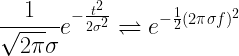
In digital communications, Gaussian Filters are employed in Gaussian Minimum Shift Keying – GMSK (used in GSM technology) and Gaussian Frequency Shift Keying (GFSK). Two dimensional Gaussian Filters are used in Image processing to produce Gaussian blurs. The impulse response of a Gaussian Filter is Gaussian. Gaussian Filters give no overshoot with minimal rise and fall time when excited with a step function. Gaussian Filter has minimum group delay. The impulse response of a Gaussian Filter is written as a Gaussian Function as follows
The Fourier Transform of a Gaussian pulse preserves its shape.
The above derivation makes use of the following result from complex analysis theory and the property of Gaussian function – total area under Gaussian function integrates to 1.
By change of variable, let ( ).
Thus, the Fourier Transform of a Gaussian pulse is a Gaussian Pulse.
Gaussian Pulse – Fourier Transform using FFT (Matlab & Python):
The following code generates a Gaussian Pulse with ( ). The Discrete Fourier Transform of this digitized version of Gaussian Pulse is plotted with the help of (FFT) function in Matlab.
fs=80; %sampling frequency
sigma=0.1;
t=-0.5:1/fs:0.5; %time base

variance=sigma^2;
x=1/(sqrt(2*pi*variance))*(exp(-t.^2/(2*variance)));
subplot(2,1,1)
plot(t,x,'b');
title(['Gaussian Pulse \sigma=', num2str(sigma),'s']);
xlabel('Time(s)');
ylabel('Amplitude');

L=length(x);
NFFT = 1024;
X = fftshift(fft(x,NFFT));
Pxx=X.*conj(X)/(NFFT*NFFT); %computing power with proper scaling
f = fs*(-NFFT/2:NFFT/2-1)/NFFT; %Frequency Vector

subplot(2,1,2)
plot(f,abs(X)/fs,'r');
title('Magnitude of FFT');
xlabel('Frequency (Hz)')
ylabel('Magnitude |X(f)|');
xlim([-10 10])
Figure 1: Gaussian pulse and its FFT (magnitude)
Double Sided and Single Power Spectral Density using FFT:
Next, the Power Spectral Density (PSD) of the Gaussian pulse is constructed using the FFT. PSD describes the power contained at each frequency component of the given signal. Double Sided power spectral density is plotted first, followed by single sided power spectral density plot (retaining only the positive frequency side of the spectrum).
Pxx=X.*conj(X)/(L*L); %computing power with proper scaling
figure;
plot(f,10*log10(Pxx),'r');
title('Double Sided - Power Spectral Density');
xlabel('Frequency (Hz)')
ylabel('Power Spectral Density- P_{xx} dB/Hz');
Figure 2: Double sided power spectral density of Gaussian pulse
X = fft(x,NFFT);
X = X(1:NFFT/2+1);%Throw the samples after NFFT/2 for single sided plot
Pxx=X.*conj(X)/(L*L);
f = fs*(0:NFFT/2)/NFFT; %Frequency Vector
figure;
plot(f,10*log10(Pxx),'r');
title('Single Sided - Power Spectral Density');
xlabel('Frequency (Hz)')
ylabel('Power Spectral Density- P_{xx} dB/Hz');
Numerous texts are available to explain the basics of Discrete Fourier Transform and its very efficient implementation – Fast Fourier Transform (FFT). Often we are confronted with the need to generate simple, standard signals (sine, cosine, Gaussian pulse, square wave, isolated rectangular pulse, exponential decay, chirp signal) for simulation purpose. I intend to show (in a series of articles) how these basic signals can be generated in Matlab and how to represent them in frequency domain using FFT.
An isolated rectangular pulse of amplitude A and duration T is represented mathematically as
where
The Fourier transform of isolated rectangular pulse g(t) is
where, the sinc function is given by
Thus, the Fourier Transform pairs are
The Fourier Transform describes the spectral content of the signal at various frequencies. For a given signal g(t), the Fourier Transform is given by
where, the absolute value gives the magnitude of the frequency components (amplitude spectrum) and are their corresponding phase (phase spectrum) . For the rectangular pulse, the amplitude spectrum is given as
The amplitude spectrum peaks at f=0 with value equal to AT. The nulls of the spectrum occur at integral multiples of 1/T, i.e, ( )
Generating an isolated rectangular pulse in Matlab:
An isolated rectangular pulse of unit amplitude and width w (the factor T in equations above ) can be generated easily with the help of in-built function – rectpuls(t,w) command in Matlab. As an example, a unit amplitude rectangular pulse of duration is generated.
fs=500; %sampling frequency
T=0.2; %width of the rectangule pulse in seconds

t=-0.5:1/fs:0.5; %time base

x=rectpuls(t,T); %generating the square wave

plot(t,x,'k');
title(['Rectangular Pulse width=', num2str(T),'s']);
xlabel('Time(s)');
ylabel('Amplitude');
Amplitude spectrum using FFT:
Matlab’s FFT function is utilized for computing the Discrete Fourier Transform (DFT). The magnitude of FFT is plotted. From the following plot, it can be noted that the amplitude of the peak occurs at f=0 with peak value . The nulls in the spectrum are located at ().
L=length(x);
NFFT = 1024;
X = fftshift(fft(x,NFFT)); %FFT with FFTshift for both negative & positive frequencies
f = fs*(-NFFT/2:NFFT/2-1)/NFFT; %Frequency Vector

figure;
plot(f,abs(X)/(L),'r');
title('Magnitude of FFT');
xlabel('Frequency (Hz)')
ylabel('Magnitude |X(f)|');
Power spectral density (PSD) using FFT:
The distribution of power among various frequency components is plotted next. The first plot shows the double-side Power Spectral Density which includes both positive and negative frequency axis. The second plot describes the PSD only for positive frequency axis (as the response is just the mirror image of negative frequency axis).
figure;
Pxx=X.*conj(X)/(L*L); %computing power with proper scaling
plot(f,10*log10(Pxx),'r');
title('Double Sided - Power Spectral Density');
xlabel('Frequency (Hz)')
ylabel('Power Spectral Density- P_{xx} dB/Hz');
X = fft(x,NFFT);
X = X(1:NFFT/2+1);%Throw the samples after NFFT/2 for single sided plot
Pxx=X.*conj(X)/(L*L);
f = fs*(0:NFFT/2)/NFFT; %Frequency Vector
plot(f,10*log10(Pxx),'r');
title('Single Sided - Power Spectral Density');
xlabel('Frequency (Hz)')
ylabel('Power Spectral Density- P_{xx} dB/Hz');
Magnitude and phase spectrum:
The phase spectrum of the rectangular pulse manifests as series of pulse trains bounded between 0 and , provided the rectangular pulse is symmetrically centered around sample zero. This is explained in the reference here and the demo below.
clearvars;
x = [ones(1,7) zeros(1,127-13) ones(1,6)];
subplot(3,1,1); plot(x,'k');
title('Rectangular Pulse'); xlabel('Sample#'); ylabel('Amplitude');

NFFT = 127;
X = fftshift(fft(x,NFFT)); %FFT with FFTshift for both negative & positive frequencies
f = (-NFFT/2:NFFT/2-1)/NFFT; %Frequency Vector

subplot(3,1,2); plot(f,abs(X),'r');
title('Magnitude Spectrum'); xlabel('Frequency (Hz)'); ylabel('|X(f)|');

subplot(3,1,3); plot(f,atan2(imag(X),real(X)),'r');
title('Phase Spectrum'); xlabel('Frequency (Hz)'); ylabel('\angle X(f)');
Note: There is a rating embedded within this post, please visit this post to rate it.
Numerous texts are available to explain the basics of Discrete Fourier Transform and its very efficient implementation – Fast Fourier Transform (FFT). Often we are confronted with the need to generate simple, standard signals (sine, cosine, Gaussian pulse, squarewave, isolated rectangular pulse, exponential decay, chirp signal) for simulation purpose. I intend to show (in a series of articles) how these basic signals can be generated in Matlab and how to represent them in frequency domain using FFT.
The most logical way of transmitting information across a communication channel is through a stream of square pulse – a distinct pulse for ‘0‘ and another for ‘1‘. Digital signals are graphically represented as square waves with certain symbol/bit period. Square waves are also used universally in switching circuits, as clock signals synchronizing various blocks of digital circuits, as reference clock for a given system domain and so on.
Square wave manifests itself as a wide range of harmonics in frequency domain and therefore can cause electromagnetic interference. Square waves are periodic and contain odd harmonics when expanded as Fourier Series (where as signals like saw-tooth and other real word signals contain harmonics at all integer frequencies). Since a square wave literally expands to infinite number of odd harmonic terms in frequency domain, approximation of square wave is another area of interest. The number of terms of its Fourier Series expansion, taken for approximating the square wave is often seen as Gibbs Phenomenon, which manifests as ringing effect at the corners of the square wave in time domain (visual explanation here).
True Square waves are a special class of rectangular waves with 50% duty cycle. Varying the duty cycle of a rectangular wave leads to pulse width modulation, where the information is conveyed by changing the duty-cycle of each transmitted rectangular wave.
How to generate a square wave in Matlab
If you know the trick of generating a sine wave in Matlab, the task is pretty much simple. Square wave is generated using “square” function in Matlab. The command sytax – square(t,dutyCycle) – generates a square wave with period for the given time base. The command behaves similar to “sin” command (used for generating sine waves), but in this case it generates a square wave instead of a sine wave. The argument – dutyCycle is optional and it defines the desired duty cycle of the square wave. By default (when the dutyCycle argument is not supplied) the square wave is generated with (50%) duty cycle.
f=10; %frequency of sine wave in Hz
overSampRate=30; %oversampling rate
fs=overSampRate*f; %sampling frequency
duty_cycle=50; % Square wave with 50% Duty cycle (default)
nCyl = 5; %to generate five cycles of sine wave

t=0:1/fs:nCyl*1/f; %time base

x=square(2*pi*f*t,duty_cycle); %generating the square wave

plot(t,x,'k');
title(['Square Wave f=', num2str(f), 'Hz']);
xlabel('Time(s)');
ylabel('Amplitude');
Power Spectral Density using FFT
Let’s check out how the generated square wave will look in frequency domain. The Fast Fourier Transform (FFT) is utilized here. As discussed in the article here, there are numerous ways to plot the response of FFT. Single Sided power spectral density is plotted first, followed by the Double-sided power spectral density.
Single Sided Power Spectral Density
X = fft(x,NFFT);
X = X(1:NFFT/2+1);%Throw the samples after NFFT/2 for single sided plot
Pxx=X.*conj(X)/(NFFT*L);
f = fs*(0:NFFT/2)/NFFT; %Frequency Vector

plot(f,10*log10(Pxx),'r');
title('Single Sided Power Spectral Density');
xlabel('Frequency (Hz)')
ylabel('Power Spectral Density- P_{xx} dB/Hz');
ylim([-45 -5])
Double Sided Power Spectral Density
L=length(x);
NFFT = 1024;
X = fftshift(fft(x,NFFT));
Pxx=X.*conj(X)/(NFFT*L); %computing power with proper scaling
f = fs*(-NFFT/2:NFFT/2-1)/NFFT; %Frequency Vector

plot(f,10*log10(Pxx),'r');
title('Double Sided Power Spectral Density');
xlabel('Frequency (Hz)')
ylabel('Power Spectral Density- P_{xx} dB/Hz');
Note: There is a rating embedded within this post, please visit this post to rate it.
Key focus: Learn how to plot FFT of sine wave and cosine wave using Matlab. Understand FFTshift. Plot one-sided, double-sided and normalized spectrum.
Introduction
Numerous texts are available to explain the basics of Discrete Fourier Transform and its very efficient implementation – Fast Fourier Transform (FFT). Often we are confronted with the need to generate simple, standard signals (sine, cosine, Gaussian pulse, squarewave, isolated rectangular pulse, exponential decay, chirp signal) for simulation purpose. I intend to show (in a series of articles) how these basic signals can be generated in Matlab and how to represent them in frequency domain using FFT. If you are inclined towards Python programming, visit here.
In order to generate a sine wave in Matlab, the first step is to fix the frequency of the sine wave. For example, I intend to generate a f=10 Hz sine wave whose minimum and maximum amplitudes are and respectively. Now that you have determined the frequency of the sinewave, the next step is to determine the sampling rate. Matlab is a software that processes everything in digital. In order to generate/plot a smooth sine wave, the sampling rate must be far higher than the prescribed minimum required sampling rate which is at least twice the frequency – as per Nyquist Shannon Theorem. A oversampling factor of is chosen here – this is to plot a smooth continuous-like sine wave (If this is not the requirement, reduce the oversampling factor to desired level). Thus the sampling rate becomes . If a phase shift is desired for the sine wave, specify it too.
f=10; %frequency of sine wave
overSampRate=30; %oversampling rate
fs=overSampRate*f; %sampling frequency
phase = 1/3*pi; %desired phase shift in radians
nCyl = 5; %to generate five cycles of sine wave

t=0:1/fs:nCyl*1/f; %time base

x=sin(2*pi*f*t+phase); %replace with cos if a cosine wave is desired
plot(t,x);
title(['Sine Wave f=', num2str(f), 'Hz']);
xlabel('Time(s)');
ylabel('Amplitude');
Representing in Frequency Domain
Representing the given signal in frequency domain is done via Fast Fourier Transform (FFT) which implements Discrete Fourier Transform (DFT) in an efficient manner. Usually, power spectrum is desired for analysis in frequency domain. In a power spectrum, power of each frequency component of the given signal is plotted against their respective frequency. The command computes the -point DFT. The number of points – – in the DFT computation is taken as power of (2) for facilitating efficient computation with FFT. A value of is chosen here. It can also be chosen as next power of 2 of the length of the signal.
Different representations of FFT:
Since FFT is just a numeric computation of -point DFT, there are many ways to plot the result.
1. Plotting raw values of DFT:
The x-axis runs from to – representing sample values. Since the DFT values are complex, the magnitude of the DFT is plotted on the y-axis. From this plot we cannot identify the frequency of the sinusoid that was generated.
2. FFT plot – plotting raw values against Normalized Frequency axis:
In the next version of plot, the frequency axis (x-axis) is normalized to unity. Just divide the sample index on the x-axis by the length of the FFT. This normalizes the x-axis with respect to the sampling rate . Still, we cannot figure out the frequency of the sinusoid from the plot.
3. FFT plot – plotting raw values against normalized frequency (positive & negative frequencies):
As you know, in the frequency domain, the values take up both positive and negative frequency axis. In order to plot the DFT values on a frequency axis with both positive and negative values, the DFT value at sample index has to be centered at the middle of the array. This is done by using function in Matlab. The x-axis runs from to where the end points are the normalized ‘folding frequencies’ with respect to the sampling rate .
4. FFT plot – Absolute frequency on the x-axis Vs Magnitude on Y-axis:
Here, the normalized frequency axis is just multiplied by the sampling rate. From the plot below we can ascertain that the absolute value of FFT peaks at and . Thus the frequency of the generated sinusoid is . The small side-lobes next to the peak values at and are due to spectral leakage.
5. Power Spectrum – Absolute frequency on the x-axis Vs Power on Y-axis:
The following is the most important representation of FFT. It plots the power of each frequency component on the y-axis and the frequency on the x-axis. The power can be plotted in linear scale or in log scale. The power of each frequency component is calculated as Where is the frequency domain representation of the signal . In Matlab, the power has to be calculated with proper scaling terms (since the length of the signal and transform length of FFT may differ from case to case).
NFFT=1024;
L=length(x);
X=fftshift(fft(x,NFFT));
Px=X.*conj(X)/(NFFT*L); %Power of each freq components
fVals=fs*(-NFFT/2:NFFT/2-1)/NFFT;
plot(fVals,Px,'b');
title('Power Spectral Density');
xlabel('Frequency (Hz)')
ylabel('Power');
NFFT=1024;
L=length(x);
X=fftshift(fft(x,NFFT));
Px=X.*conj(X)/(NFFT*L); %Power of each freq components
fVals=fs*(-NFFT/2:NFFT/2-1)/NFFT;
plot(fVals,10*log10(Px),'b');
title('Power Spectral Density');
xlabel('Frequency (Hz)')
ylabel('Power');
6. Power Spectrum – One-Sided frequencies
In this type of plot, the negative frequency part of x-axis is omitted. Only the FFT values corresponding to to sample points of -point DFT are plotted. Correspondingly, the normalized frequency axis runs between to . The absolute frequency (x-axis) runs from to .
L=length(x);
NFFT=1024;
X=fft(x,NFFT);
Px=X.*conj(X)/(NFFT*L); %Power of each freq components
fVals=fs*(0:NFFT/2-1)/NFFT;
plot(fVals,Px(1:NFFT/2),'b','LineSmoothing','on','LineWidth',1);
title('One Sided Power Spectral Density');
xlabel('Frequency (Hz)')
ylabel('PSD');
Rate this article: Note: There is a rating embedded within this post, please visit this post to rate it.
A random process (or signal for your visualization) with a constant power spectral density (PSD) function is a white noise process.
Power Spectral Density
Power Spectral Density function (PSD) shows how much power is contained in each of the spectral component. For example, for a sine wave of fixed frequency, the PSD plot will contain only one spectral component present at the given frequency. PSD is an even function and so the frequency components will be mirrored across the Y-axis when plotted. Thus for a sine wave of fixed frequency, the double sided plot of PSD will have two components – one at +ve frequency and another at –ve frequency of the sine wave. (Know how to plot PSD/FFT in Python & in Matlab)
Gaussian and Uniform White Noise:
A white noise signal (process) is constituted by a set of independent and identically distributed (i.i.d) random variables. In discrete sense, the white noise signal constitutes a series of samples that are independent and generated from the same probability distribution. For example, you can generate a white noise signal using a random number generator in which all the samples follow a given Gaussian distribution. This is called White Gaussian Noise (WGN) or Gaussian White Noise. Similarly, a white noise signal generated from a Uniform distribution is called Uniform White Noise.
Gaussian Noise and Uniform Noise are frequently used in system modelling. In modelling/simulation, white noise can be generated using an appropriate random generator. White Gaussian Noise can be generated using randn function in Matlab which generates random numbers that follow a Gaussian distribution. Similarly, rand function can be used to generate Uniform White Noise in Matlab that follows a uniform distribution. When the random number generators are used, it generates a series of random numbers from the given distribution. Let’s take the example of generating a White Gaussian Noise of length 10 using randn function in Matlab – with zero mean and standard deviation=1.
This simply generates 10 random numbers from the standard normal distribution. As we know that a white process is seen as a random process composing several random variables following the same Probability Distribution Function (PDF). The 10 random numbers above are generated from the same PDF (standard normal distribution). This condition is called “identically distributed” condition. The individual samples given above are “independent” of each other. Furthermore, each sample can be viewed as a realization of one random variable. In effect, we have generated a random process that is composed of realizations of 10 random variables. Thus, the process above is constituted from “independent identically distributed” (i.i.d) random variables.
Strictly and weakly defined white noise:
Since the white noise process is constructed from i.i.d random variable/samples, all the samples follow the same underlying probability distribution function (PDF). Thus, the Joint Probability Distribution function of the process will not change with any shift in time. This is called a stationary process. Hence, this noise is a stationary process. As with a stationary process which can be classified as Strict Sense Stationary (SSS) and Wide Sense Stationary (WSS) processes, we can have white noise that is SSS and white noise that is WSS. Correspondingly they can be called strictly defined white noise signal and weakly defined white noise signal.
What’s with Covariance Function/Matrix ?
A white noise signal, denoted by \(x(t)\), is defined in weak sense is a more practical condition. Here, the samples are statistically uncorrelated and identically distributed with some variance equal to \(\sigma^2\). This condition is specified by using a covariance function as
\[COV \left(x_i, x_j \right) = \begin{cases} \sigma^2, & \quad i = j \\ 0, & \quad i \neq j \end{cases}\]
Why do we need a covariance function? Because, we are dealing with a random process that is composed of \(n\) random variables (10 variables in the modelling example above). Such a process is viewed as multivariate random vector or multivariate random variable.
For multivariate random variables, Covariance function specified how each of the \(n\) variables in the given random process behaves with respect to each other. Covariance function generalizes the notion of variance to multiple dimensions.
The above equation when represented in the matrix form gives the covariance matrix of the white noise random process. Since the random variables in this process are statistically uncorrelated, the covariance function contains values only along the diagonal.
The matrix above indicates that only the auto-correlation function exists for each random variable. The cross-correlation values are zero (samples/variables are statistically uncorrelated with respect to each other). The diagonal elements are equal to the variance and all other elements in the matrix are zero.The ensemble auto-correlation function of the weakly defined white noise is given by This indicates that the auto-correlation function of weakly defined white noise process is zero everywhere except at lag \(\tau=0\).
\[R_{xx}(\tau) = E \left[ x(t) x^*(t-\tau)\right] = \sigma^2 \delta (\tau)\]
Wiener-Khintchine Theorem states that for Wide Sense Stationary Process (WSS), the power spectral density function \(S_{xx}(f)\) of a random process can be obtained by Fourier Transform of auto-correlation function of the random process. In continuous time domain, this is represented as
\[S_{xx}(f) = F \left[R_{xx}(\tau) \right] = \int_{-\infty}^{\infty} R_{xx} (\tau) e ^{- j 2 \pi f \tau} d \tau\]
For the weakly defined white noise process, we find that the mean is a constant and its covariance does not vary with respect to time. This is a sufficient condition for a WSS process. Thus we can apply Weiner-Khintchine Theorem. Therefore, the power spectral density of the weakly defined white noise process is constant (flat) across the entire frequency spectrum (Figure 1). The value of the constant is equal to the variance or power of the noise signal.
\[S_{xx}(f) = F \left[R_{xx}(\tau) \right] = \int_{-\infty}^{\infty} \sigma^2 \delta (\tau) e ^{- j 2 \pi f \tau} d \tau = \sigma^2 \int_{-\infty}^{\infty} \delta (\tau) e ^{- j 2 \pi f \tau} = \sigma^2\]
Figure 1: Weiner-Khintchine theorem illustrated
Testing the characteristics of White Gaussian Noise in Matlab:
Generate a Gaussian white noise signal of length \(L=100,000\) using the randn function in Matlab and plot it. Let’s assume that the pdf is a Gaussian pdf with mean \(\mu=0\) and standard deviation \(\sigma=2\). Thus the variance of the Gaussian pdf is \(\sigma^2=4\). The theoretical PDF of Gaussian random variable is given by
subplot(2,1,2)
n=100; %number of Histrogram bins
[f,x]=hist(X,n);
bar(x,f/trapz(x,f)); hold on;
%Theoretical PDF of Gaussian Random Variable
g=(1/(sqrt(2*pi)*sigma))*exp(-((x-mu).^2)/(2*sigma^2));
plot(x,g);hold off; grid on;
title('Theoretical PDF and Simulated Histogram of White Gaussian Noise');
legend('Histogram','Theoretical PDF');
xlabel('Bins');
ylabel('PDF f_x(x)');
Figure 3: Plot of simulated & theoretical PDF for Gaussian RV
Compute the auto-correlation function of the white noise. The computed auto-correlation function has to be scaled properly. If the ‘xcorr’ function (inbuilt in Matlab) is used for computing the auto-correlation function, use the ‘biased’ argument in the function to scale it properly.
figure();
Rxx=1/L*conv(flipud(X),X);
lags=(-L+1):1:(L-1);

%Alternative method
%[Rxx,lags] =xcorr(X,'biased');
%The argument 'biased' is used for proper scaling by 1/L
%Normalize auto-correlation with sample length for proper scaling

plot(lags,Rxx);
title('Auto-correlation Function of white noise');
xlabel('Lags')
ylabel('Correlation')
grid on;
Figure 4: Autocorrelation function of generated noise
Simulating the PSD:
Simulating the Power Spectral Density (PSD) of the white noise is a little tricky business. There are two issues here 1) The generated samples are of finite length. This is synonymous to applying truncating an infinite series of random samples. This implies that the lags are defined over a fixed range. ( FFT and spectral leakage – an additional resource on this topic can be found here) 2) The random number generators used in simulations are pseudo-random generators. Due these two reasons, you will not get a flat spectrum of psd when you apply Fourier Transform over the generated auto-correlation values.The wavering effect of the psd can be minimized by generating sufficiently long random signal and averaging the psd over several realizations of the random signal.
Simulating Gaussian White Noise as a Multivariate Gaussian Random Vector:
To verify the power spectral density of the white noise, we will use the approach of envisaging the noise as a composite of \(N\) Gaussian random variables. We want to average the PSD over \(L\) such realizations. Since there are \(N\) Gaussian random variables (\(N\) individual samples) per realization, the covariance matrix \( C_{xx}\) will be of dimension \(N \times N\). The vector of mean for this multivariate case will be of dimension \(1 \times N\).
Cholesky decomposition of covariance matrix gives the equivalent standard deviation for the multivariate case. Cholesky decomposition can be viewed as square root operation. Matlab’s randn function is used here to generate the multi-dimensional Gaussian random process with the given mean matrix and covariance matrix.
%Verifying the constant PSD of White Gaussian Noise Process
%with arbitrary mean and standard deviation sigma

mu=0; %Mean of each realization of Noise Process
sigma=2; %Sigma of each realization of Noise Process

L = 1000; %Number of Random Signal realizations to average
N = 1024; %Sample length for each realization set as power of 2 for FFT

%Generating the Random Process - White Gaussian Noise process
MU=mu*ones(1,N); %Vector of mean for all realizations
Cxx=(sigma^2)*diag(ones(N,1)); %Covariance Matrix for the Random Process
R = chol(Cxx); %Cholesky of Covariance Matrix
%Generating a Multivariate Gaussian Distribution with given mean vector and
%Covariance Matrix Cxx
z = repmat(MU,L,1) + randn(L,N)*R;
Compute PSD of the above generated multi-dimensional process and average it to get a smooth plot.
%By default, FFT is done across each column - Normal command fft(z)
%Finding the FFT of the Multivariate Distribution across each row
%Command - fft(z,[],2)
Z = 1/sqrt(N)*fft(z,[],2); %Scaling by sqrt(N);
Pzavg = mean(Z.*conj(Z));%Computing the mean power from fft

normFreq=[-N/2:N/2-1]/N;
Pzavg=fftshift(Pzavg); %Shift zero-frequency component to center of spectrum
plot(normFreq,10*log10(Pzavg),'r');
axis([-0.5 0.5 0 10]); grid on;
ylabel('Power Spectral Density (dB/Hz)');
xlabel('Normalized Frequency');
title('Power spectral density of white noise');
Figure 5: Power spectral density of generated noise
The PSD plot of the generated noise shows almost fixed power in all the frequencies. In other words, for a white noise signal, the PSD is constant (flat) across all the frequencies (\(- \infty\) to \(+\infty\)). The y-axis in the above plot is expressed in dB/Hz unit. We can see from the plot that the \(constant \; power = 10 log_{10}(\sigma^2) = 10 log_{10}(4) = 6\; dB\).
Application
In channel modeling, we often come across additive white Gaussian noise (AWGN) channel. To know more about the channel model and its simulation, continue reading this article: Simulate AWGN channel in Matlab & Python.
Rate this article: Note: There is a rating embedded within this post, please visit this post to rate it.
Understand Fourier Series, Fourier Cosine Series, Fourier Sine Series, partial sums, even odd symmetry. Hands-on simulation with Matlab code given.
Fourier analysis and Fourier Synthesis:
Fourier analysis – a term named after the French mathematician Joseph Fourier, is the process of breaking down a complex function and expressing it as a combination of simpler functions. The reverse process of combining simpler functions to reconstruct the complex function is termed as Fourier Synthesis.
Mostly, the simpler functions are chosen to be sine and cosine functions. Thus, the term “Fourier analysis” expresses a complex function in terms of sine and cosine terms and the term “Fourier Analysis” reconstructs the complex function from the sine and cosine terms.
Frequency is the measure of number of repetitive occurrences of a particular event. By definition, a sine wave is a smooth curve that repeats at a certain frequency. Thus, the term “frequency” and sine are almost synonymous. A cosine wave is also a sine wave but with 90* phase shift. Therefore, when you talk about sine and cosine functions, you are taking in terms of “frequencies”. That is why in signal processing, the Fourier analysis is applied in frequency (or spectrum) analysis.
Fourier series, Continuous Fourier Transform, Discrete Fourier Transform, and Discrete Time Fourier Transform are some of the variants of Fourier analysis.
Fourier series:
Applied on functions that are periodic. A periodic function is broken down and expressed in terms of sine and cosine terms. In mathematics, the term “series” represents a sum of sequence of numbers. For example we can make a series with a sequence of numbers that follows Geometric Progression (common ratio between the numbers)
Common ratio =3 : 1+ 3 + 9 + 27 + …
An infinite series is a series that has infinite number of terms. If the elements of the infinite series has a common ratio less than 1, then there is a possibility of the sum converging at a particular value. Fourier series falls under the category of trigonometric infinite series, where the individual elements of the series are expressed trigonometrically. The construct of the Fourier series is given by
Here f(x) is the complex periodic function we wish to break down in terms of sine and cosine basis functions. The coefficients a0, a1,… and b1, b2,… can be found by
Functions and Symmetry:
It is necessary to classify the functions according to its symmetry properties. Doing so will save computation time and effort. Functions either fall into odd symmetry or even symmetry or no symmetry category. Symmetry can be ascertained by plotting the function in a graph paper and folding it along the y axis. Symmetry of a function is always with respect to y axis.
Even Symmetry:
Figure 1: A function exhibiting even-symmetry
Mathematically depicted as f(x) = f(-x). The value of the given function f(x) at a given positive value x is same at corresponding negative value –x. If plotted on a graph paper and folded along the y-axis, the left half and the right half of the function matches with each other (mirror image).
For even symmetry functions, only the cosine terms exist in Fourier Series expansion. The bn coefficients vanishes all-together (i.e, no sine basis). This leads to what is called Fourier Cosine Series.
Odd Symmetry:
Mathematically depicted as f(x) = -f(-x). The value of the given function f(x) at a given positive value x is same but with a sign change at corresponding negative value –x. If plotted on a graph paper and folded along the y-axis, the left half of the graph will look like inverted (upside down) mirror image of the right half.
Figure 2: A function exhibiting odd-symmetry
For odd symmetry functions, only the sine terms exists in Fourier Series expansion. The an coefficients vanishes all-together (no cosine basis). This leads to what is called Fourier Sine Series.
Thus, knowing the symmetry could save us a lots of computation time and effort, as we do not have to calculate half the number of coefficients if symmetry exists.
Table: Fourier Series and Function Symmetry
Partial Sum and Convergence of Fourier Series:
Fourier Series is a class of infinite series, meaning that there are infinite terms in the expansion.We cannot go on calculating the terms indefinitely. To decompose a complex function using Fourier Series expansion, one has to limit the number of terms we wish to obtain and this process affects convergence. Convergence is based on certain criteria. There exists a separate branch of mathematics called Classical Harmonic Analysis that deals with this subject. Convergence is usually calculated over a partial sum – the sum of all terms upto which we have calculated the coefficients.
Example:
Consider the following periodic function :
Investigation of the function plot reveals that this function exhibits anti-symmetry (odd symmetry). So it is enough if we compute only the sine terms in the Fourier expansion.
Figure 3: Example for odd-symmetry
Computing the Fourier Sine Series:
Thus the complete Fourier expansion of the given function f(x) is given by
Note that the sine term vanishes when n is even (n=0,2,4,…,). Thus the above expansion can be simplified to
Matlab Simulation:
The following Matlab simulation computes the Fourier series expansion of the above mentioned function. The partial sum is plotted till an error criteria is satisfied.
The function f(x) either stays at +1 or at -1. The partial sum is calculated for each iteration and compared with either +1 or -1 and till the error reaches a small value of 0.01.
%Author Mathuranathan Viswanathan for https://gaussianwaves.com
%Creative Commons CC-BY-NC-SA
%If you use this piece of code you must attribute the author

clearvars;clc;
time=linspace(-pi,pi,1000);
partial_sum=0;

%Complex Function represented in terms of time and amplitude value
t=[-pi,-pi,0,0,pi,pi];
value=[0,-1,-1,1,1,-1];
handle1=line(t,value,'color','r','linewidth',2);
grid on;hold on;
axis([-pi pi -1.5 1.5])
%Since the given complex function exhibits odd periodic extension
%only Bn term is valid with n=1,3,5,...

for n=1:2:200 %Odd terms to consider for partial sums
    %Plot 1 period of the given function
    partial_sum=partial_sum+(4/(n*pi))*sin(n*time); %Fourier Series Expansion using Sine terms
    error=mean((abs(partial_sum)-1).^2); %Error Criteria
    handle2=plot(time,partial_sum,'k','linewidth',2);
    title(['Square Wave Partial Sum:  n = ',num2str(n),'  Error = ',num2str(error)])
    pause
    set(handle2,'Visible','off');
    if error<0.01
        break
    end
end
The plots below shows that the error gets minimized as more and more terms are included in the series expansion.
In the first plot, the original square wave (red color) is decomposed into first three terms (n=3) of the Fourier Series. The plot in black color shows how the reconstructed (Fourier Synthesis) signal will look like if the three terms are combined together. As you progress further by increasing the number of terms ( n= 7, 15, 41, …) the plot in the black color increasingly resembles the original square wave.
Note the ringing effect at the corners of the black plot as the number of decomposed terms (n) is increased. This phenomenon is called Gibbs Phenomenon. Remember that the Fourier Series is an infinite series with indefinite number of terms. Since we cannot calculate all the infinite number of terms we have to stop at some point. This truncation of the number of decomposed terms leads to Gibbs Phenomenon. Read more on Gibss Phenomenon and its simulation in Matlab here.
Rate this article: Note: There is a rating embedded within this post, please visit this post to rate it.
This website uses cookies to improve your experience while you navigate through the website. Out of these, the cookies that are categorized as necessary are stored on your browser as they are essential for the working of basic functionalities of the website. We also use third-party cookies that help us analyze and understand how you use this website. These cookies will be stored in your browser only with your consent. You also have the option to opt-out of these cookies. But opting out of some of these cookies may affect your browsing experience.
Necessary cookies are absolutely essential for the website to function properly. These cookies ensure basic functionalities and security features of the website, anonymously.
Cookie
Duration
Description
cookielawinfo-checbox-analytics
11 months
This cookie is set by GDPR Cookie Consent plugin. The cookie is used to store the user consent for the cookies in the category "Analytics".
cookielawinfo-checbox-analytics
11 months
This cookie is set by GDPR Cookie Consent plugin. The cookie is used to store the user consent for the cookies in the category "Analytics".
cookielawinfo-checbox-functional
11 months
The cookie is set by GDPR cookie consent to record the user consent for the cookies in the category "Functional".
cookielawinfo-checbox-functional
11 months
The cookie is set by GDPR cookie consent to record the user consent for the cookies in the category "Functional".
cookielawinfo-checbox-others
11 months
This cookie is set by GDPR Cookie Consent plugin. The cookie is used to store the user consent for the cookies in the category "Other.
cookielawinfo-checbox-others
11 months
This cookie is set by GDPR Cookie Consent plugin. The cookie is used to store the user consent for the cookies in the category "Other.
cookielawinfo-checkbox-necessary
11 months
This cookie is set by GDPR Cookie Consent plugin. The cookies is used to store the user consent for the cookies in the category "Necessary".
cookielawinfo-checkbox-performance
11 months
This cookie is set by GDPR Cookie Consent plugin. The cookie is used to store the user consent for the cookies in the category "Performance".
viewed_cookie_policy
11 months
The cookie is set by the GDPR Cookie Consent plugin and is used to store whether or not user has consented to the use of cookies. It does not store any personal data.
Functional cookies help to perform certain functionalities like sharing the content of the website on social media platforms, collect feedbacks, and other third-party features.
Performance cookies are used to understand and analyze the key performance indexes of the website which helps in delivering a better user experience for the visitors.
Analytical cookies are used to understand how visitors interact with the website. These cookies help provide information on metrics the number of visitors, bounce rate, traffic source, etc.


![\begin{aligned} G(f) &=F[g(t)]\\ &= \int_{-\infty }^{\infty } g(t)e^{-j2\pi ft}\, dt\\ &= \frac{1}{\sigma \sqrt{2 \pi } } \int_{-\infty }^{\infty } e^{- \frac{t^2}{2 \sigma^2}}e^{-j2\pi ft}\, dt\\ &=\frac{1}{\sigma \sqrt{2 \pi } } \int_{-\infty }^{\infty } e^{- \frac{1}{2 \sigma^2}\left[t^2+j4 \pi \sigma^2 ft \right]}\, dt\\ &=\frac{1}{\sigma \sqrt{2 \pi } } \int_{-\infty }^{\infty } e^{- \frac{1}{2 \sigma^2}\left[t^2+j4 \pi \sigma^2 ft + (j 2 \pi \sigma^2 f)^2 - (j 2 \pi \sigma^2 f)^2\right]}\, dt\\ &=e^{ \frac{1}{2 \sigma^2}(j 2 \pi \sigma^2 f)^2}\frac{1}{\sigma \sqrt{2 \pi } } \int_{-\infty }^{\infty } e^{- \frac{1}{2 \sigma^2}\left[t+j 2 \pi \sigma^2 f \right]^2}\, dt\\ &=e^{ \frac{1}{2 \sigma^2}(j 2 \pi \sigma^2 f)^2}=e^{ - \frac{1}{2}( 2 \pi \sigma f)^2}\end{aligned}](https://s0.wp.com/latex.php?latex=%5Cbegin%7Baligned%7D+G%28f%29+%26%3DF%5Bg%28t%29%5D%5C%5C+%26%3D+%5Cint_%7B-%5Cinfty+%7D%5E%7B%5Cinfty+%7D+g%28t%29e%5E%7B-j2%5Cpi+ft%7D%5C%2C+dt%5C%5C+%26%3D+%5Cfrac%7B1%7D%7B%5Csigma+%5Csqrt%7B2+%5Cpi+%7D+%7D+%5Cint_%7B-%5Cinfty+%7D%5E%7B%5Cinfty+%7D+e%5E%7B-+%5Cfrac%7Bt%5E2%7D%7B2+%5Csigma%5E2%7D%7De%5E%7B-j2%5Cpi+ft%7D%5C%2C+dt%5C%5C+%26%3D%5Cfrac%7B1%7D%7B%5Csigma+%5Csqrt%7B2+%5Cpi+%7D+%7D+%5Cint_%7B-%5Cinfty+%7D%5E%7B%5Cinfty+%7D+e%5E%7B-+%5Cfrac%7B1%7D%7B2+%5Csigma%5E2%7D%5Cleft%5Bt%5E2%2Bj4+%5Cpi+%5Csigma%5E2+ft+%5Cright%5D%7D%5C%2C+dt%5C%5C+%26%3D%5Cfrac%7B1%7D%7B%5Csigma+%5Csqrt%7B2+%5Cpi+%7D+%7D+%5Cint_%7B-%5Cinfty+%7D%5E%7B%5Cinfty+%7D+e%5E%7B-+%5Cfrac%7B1%7D%7B2+%5Csigma%5E2%7D%5Cleft%5Bt%5E2%2Bj4+%5Cpi+%5Csigma%5E2+ft+%2B+%28j+2+%5Cpi+%5Csigma%5E2+f%29%5E2+-+%28j+2+%5Cpi+%5Csigma%5E2+f%29%5E2%5Cright%5D%7D%5C%2C+dt%5C%5C+%26%3De%5E%7B+%5Cfrac%7B1%7D%7B2+%5Csigma%5E2%7D%28j+2+%5Cpi+%5Csigma%5E2+f%29%5E2%7D%5Cfrac%7B1%7D%7B%5Csigma+%5Csqrt%7B2+%5Cpi+%7D+%7D+%5Cint_%7B-%5Cinfty+%7D%5E%7B%5Cinfty+%7D+e%5E%7B-+%5Cfrac%7B1%7D%7B2+%5Csigma%5E2%7D%5Cleft%5Bt%2Bj+2+%5Cpi+%5Csigma%5E2+f+%5Cright%5D%5E2%7D%5C%2C+dt%5C%5C+%26%3De%5E%7B+%5Cfrac%7B1%7D%7B2+%5Csigma%5E2%7D%28j+2+%5Cpi+%5Csigma%5E2+f%29%5E2%7D%3De%5E%7B+-+%5Cfrac%7B1%7D%7B2%7D%28+2+%5Cpi+%5Csigma+f%29%5E2%7D%5Cend%7Baligned%7D+&bg=ffffff&fg=000&s=2&c=20201002)


![\displaystyle{\frac{1}{\sigma \sqrt{2 \pi} }\int_{-\infty }^{\infty }e^{- \frac{1}{2 \sigma^2}\left[t+j 2 \pi \sigma^2 f \right]^2}\, dt =\frac{1}{\sigma \sqrt{2 \pi } }\int_{-\infty }^{\infty }e^{- \frac{1}{2 \sigma^2} u^2}\, du =1}](https://s0.wp.com/latex.php?latex=%5Cdisplaystyle%7B%5Cfrac%7B1%7D%7B%5Csigma+%5Csqrt%7B2+%5Cpi%7D+%7D%5Cint_%7B-%5Cinfty+%7D%5E%7B%5Cinfty+%7De%5E%7B-+%5Cfrac%7B1%7D%7B2+%5Csigma%5E2%7D%5Cleft%5Bt%2Bj+2+%5Cpi+%5Csigma%5E2+f+%5Cright%5D%5E2%7D%5C%2C+dt+%3D%5Cfrac%7B1%7D%7B%5Csigma+%5Csqrt%7B2+%5Cpi+%7D+%7D%5Cint_%7B-%5Cinfty+%7D%5E%7B%5Cinfty+%7De%5E%7B-+%5Cfrac%7B1%7D%7B2+%5Csigma%5E2%7D+u%5E2%7D%5C%2C+du+%3D1%7D+&bg=ffffff&fg=000&s=2&c=20201002)