Tutorials Archives - Page 2 of 2

Interpret FFT, complex DFT, frequency bins & FFTShift

Key focus: Interpret FFT results, complex DFT, frequency bins, fftshift and ifftshift. Know how to use them in analysis using Matlab and Python.

This article is part of the following books
● Digital Modulations using Matlab : Build Simulation Models from Scratch, ISBN: 978-1521493885
● Digital Modulations using Python ISBN: 978-1712321638
● Wireless communication systems in Matlab ISBN: 979-8648350779
All books available in ebook (PDF) and Paperback formats

Four types of Fourier Transforms:

Often, one is confronted with the problem of converting a time domain signal to frequency domain and vice-versa. Fourier Transform is an excellent tool to achieve this conversion and is ubiquitously used in many applications. In signal processing, a time domain signal can be continuous or discrete and it can be aperiodic or periodic. This gives rise to four types of Fourier transforms.

From Table 1, we note note that when the signal is discrete in one domain, it will be periodic in other domain. Similarly, if the signal is continuous in one domain, it will be aperiodic (non-periodic) in another domain. For simplicity, let’s not venture into the specific equations for each of the transforms above. We will limit our discussion to DFT, that is widely available as part of software packages like Matlab, Scipy(python) etc.., however we can approximate other transforms using DFT.

Real and Complex versions of transforms

For each of the listed transforms above, there exist a real version and complex version. The real version of the transform, takes in a real numbers and gives two sets of real frequency domain points – one set representing coefficients over $cosine$ basis function and the other set representing the co-efficient over $sine$ basis function. The complex version of the transforms represent positive and negative frequencies in a single array. The complex versions are flexible that it can process both complex valued signals and real valued signals. The following figure captures the difference between real DFT and complex DFT.

Real DFT:

Consider the case of N-point $real$ DFT , it takes in N samples of (real-valued) time domain waveform $x[n]$ and gives two arrays of length $N/2+1$ each set projected on cosine and sine functions respectively.

\[\begin{align} X_{re}[k] &= \phantom{-}\frac{2}{N} \displaystyle{ \sum_{n=0}^{N-1} x[n] \cdot cos\left( \frac{2 \pi k n}{N} \right)} \\ X_{im}[k] &= -\frac{2}{N} \sum_{n=0}^{N-1} \displaystyle{ x[n] \cdot sin\left( \frac{2 \pi k n}{N} \right)} \end{align}\]

Here, the time domain index $n$ runs from $0 \rightarrow N$, the frequency domain index $k$ runs from $0 \rightarrow N/2$

The real-valued time domain signal $x [n]$ can be synthesized from the real DFT pairs as

\[x[n] = \displaystyle{ \sum_{k=0}^{N/2} X_{re}[K] \cdot cos\left( \frac{2 \pi k n}{N} \right) – X_{im}[K] \cdot sin\left( \frac{2 \pi k n}{N} \right)}\]

Caveat: When using the synthesis equation, the values $X_{re}[0]$ and $X_{re}[N/2] $ must be divided by two. This problem is due to the fact that we restrict the analysis to real-values only. These type of problems can be avoided by using complex version of DFT.

Complex DFT:

Consider the case of N-point complex DFT, it takes in N samples of complex-valued time domain waveform $x[n]$ and produces an array $X[k]$ of length N.

\[ X[k]= \displaystyle{\sum_{n=0}^{N-1} x[n] e^{-j2 \pi k n/N}}\]

The arrays values are interpreted as follows

● $X[0]$ represents DC frequency component
● Next $N/2$ terms are positive frequency components with $X[N/2]$ being the Nyquist frequency (which is equal to half of sampling frequency)
● Next $N/2-1$ terms are negative frequency components (note: negative frequency components are the phasors rotating in opposite direction, they can be optionally omitted depending on the application)

The corresponding synthesis equation (reconstruct $x[n]$ from frequency domain samples $X[k]$) is

\[x[n]= \displaystyle{ \frac{1}{N} \sum_{k=0}^{N-1} X[k] e^{j2 \pi k n/N}} \]

From these equations we can see that the real DFT is computed by projecting the signal on cosine and sine basis functions. However, the complex DFT projects the input signal on exponential basis functions (Euler’s formula connects these two concepts).

When the input signal in the time domain is real valued, the complex DFT zero-fills the imaginary part during computation (That’s its flexibility and avoids the caveat needed for real DFT). The following figure shows how to interpret the raw FFT results in Matlab that computes complex DFT. The specifics will be discussed next with an example.

Figure 2: Interpretation of frequencies in complex DFT output

Fast Fourier Transform (FFT)

The FFT function in Matlab is an algorithm published in 1965 by J.W.Cooley and J.W.Tuckey for efficiently calculating the DFT. It exploits the special structure of DFT when the signal length is a power of 2, when this happens, the computation complexity is significantly reduced. FFT length is generally considered as power of 2 – this is called $radix-2$ FFT which exploits the twiddle factors. The FFT length can be odd as used in this particular FFT implementation – Prime-factor FFT algorithm where the FFT length factors into two co-primes.

FFT is widely available in software packages like Matlab, Scipy etc.., FFT in Matlab/Scipy implements the complex version of DFT. Matlab’s FFT implementation computes the complex DFT that is very similar to above equations except for the scaling factor. For comparison, the Matlab’s FFT implementation computes the complex DFT and its inverse as

\[ \begin{align} X[k] &= \displaystyle{ \phantom {\frac{1}{N}}\sum_{n=0}^{N-1} x[n] e^{-j2 \pi k n/N}} \\ x[n] &= \displaystyle{ \frac{1}{N} \sum_{k=0}^{N-1} X[k] e^{j2 \pi k n/N}} \end{align}\]

The Matlab commands that implement the above equations are FFT and IFFT) respectively. The corresponding syntax is as follows

X = fft(x,N) %compute X[k]
x = ifft(X,N) %compute x[n]

Interpreting the FFT results

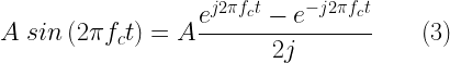
Lets assume that the $x[n]$ is the time domain cosine signal of frequency $f_c=10Hz$ that is sampled at a frequency $f_s=32*fc$ for representing it in the computer memory.

fc=10;%frequency of the carrier
fs=32*fc;%sampling frequency with oversampling factor=32
t=0:1/fs:2-1/fs;%2 seconds duration
x=cos(2*pi*fc*t);%time domain signal (real number)
subplot(3,1,1); plot(t,x);hold on; %plot the signal
title('x[n]=cos(2 \pi 10 t)'); xlabel('n'); ylabel('x[n]');

Figure 3: A 2 seconds record of 10 Hz cosine wave

Lets consider taking a $N=256$ point FFT, which is the $8^{th}$ power of $2$.

N=256; %FFT size
X = fft(x,N);%N-point complex DFT
%output contains DC at index 1, Nyquist frequency at N/2+1 th index
%positive frequencies from index 2 to N/2
%negative frequencies from index N/2+1 to N

Note: The FFT length should be sufficient to cover the entire length of the input signal. If $N$ is less than the length of the input signal, the input signal will be truncated when computing the FFT. In our case, the cosine wave is of 2 seconds duration and it will have 640 points (a $10Hz$ frequency wave sampled at 32 times oversampling factor will have $2 \times 32 \times 10 = 640$ samples in 2 seconds of the record). Since our input signal is periodic, we can safely use $N=256$ point FFT, anyways the FFT will extend the signal when computing the FFT (see additional topic on spectral leakage that explains this extension concept).

Due to Matlab’s index starting at 1, the DC component of the FFT decomposition is present at index 1.

>>X(1)
 1.1762e-14   (approximately equal to zero)

That’s pretty easy. Note that the index for the raw FFT are integers from $1 \rightarrow N$. We need to process it to convert these integers to $frequencies$. That is where the $sampling$ frequency counts.

Each point/bin in the FFT output array is spaced by the frequency resolution $\Delta f$ that is calculated as

\[ \Delta f = \frac{f_s}{N} \]

where, $f_s$ is the sampling frequency and $N$ is the FFT size that is considered. Thus, for our example, each point in the array is spaced by the frequency resolution

\[\Delta f = \frac{f_s}{N} = \frac{32*f_c}{256} = \frac{320}{256} = 1.25 Hz \]

Now, the $10 Hz$ cosine signal will leave a spike at the 8th sample ($10/1.25=8$), which is located at index 9 (See next figure).

>> abs(X(8:10)) %display samples 7 to 9
ans = 0.0000  128.0000    0.0000

Therefore, from the frequency resolution, the entire frequency axis can be computed as

%calculate frequency bins with FFT
df=fs/N %frequency resolution
sampleIndex = 0:N-1; %raw index for FFT plot
f=sampleIndex*df; %x-axis index converted to frequencies

Now we can plot the absolute value of the FFT against frequencies as

subplot(3,1,2); stem(sampleIndex,abs(X)); %sample values on x-axis
title('X[k]'); xlabel('k'); ylabel('|X(k)|');
subplot(3,1,3); plot(f,abs(X)); %x-axis represent frequencies
title('X[k]'); xlabel('frequencies (f)'); ylabel('|X(k)|');

The following plot shows the frequency axis and the sample index as it is for the complex FFT output.

Figure 4: Magnitude response from FFT output plotted against sample index (top) and computed frequencies (bottom)

After the frequency axis is properly transformed with respect to the sampling frequency, we note that the cosine signal has registered a spike at $10 Hz$. In addition to that, it has also registered a spike at $256-8=248^{th}$ sample that belongs to negative frequency portion. Since we know the nature of the signal, we can optionally ignore the negative frequencies. The sample at the Nyquist frequency ($f_s/2$) mark the boundary between the positive and negative frequencies.

>> nyquistIndex=N/2+1;
>> X(nyquistIndex-2:nyquistIndex+2).'
ans =
1.0e-13 *
  -0.2428 + 0.0404i
  -0.1897 + 0.0999i
  -0.3784          
  -0.1897 - 0.0999i
  -0.2428 - 0.0404i

Note that the complex numbers surrounding the Nyquist index are complex conjugates and they represent positive and negative frequencies respectively.

FFTShift

From the plot we see that the frequency axis starts with DC, followed by positive frequency terms which is in turn followed by the negative frequency terms. To introduce proper order in the x-axis, one can use FFTshift function Matlab, which arranges the frequencies in order: negative frequencies $\rightarrow$ DC $\rightarrow$ positive frequencies. The fftshift function need to be carefully used when $N$ is odd.

For even N, the original order returned by FFT is as follows (note: all indices below corresponds to Matlab’s index)

● $X[1]$ represents DC frequency component
● $X[2]$ to $X[N/2]$ terms are positive frequency components
● $X[N/2+1]$ is the Nyquist frequency ($F_s/2$) that is common to both positive and negative frequencies. We will consider it as part of negative frequencies to have the same equivalence with the fftshift function.
● $X[N/2+1]$ to $X[N]$ terms are considered as negative frequency components

FFTshift shifts the DC component to the center of the spectrum. It is important to remember that the Nyquist frequency at the (N/2+1)th Matlab index is common to both positive and negative frequency sides. FFTshift command puts the Nyquist frequency in the negative frequency side. This is captured in the following illustration.

Figure 5: Role of FFTShift in ordering the frequencies

Therefore, when $N$ is even, ordered frequency axis is set as

\[f = \Delta f \left[ -\frac{N}{2}:1:\frac{N}{2}-1 \right] = \frac{f_s}{N} \left[ -\frac{N}{2}:1:\frac{N}{2}-1 \right]\]

When (N) is odd, the ordered frequency axis should be set as

\[ f = \Delta f \left[ -\frac{N-1}{2}:1:\frac{N+1}{2}-1 \right] = \frac{f_s}{N} \left[ -\frac{N-1}{2}:1:\frac{N-1}{2}-1 \right]\]

The following code snippet, computes the fftshift using both the manual method and using the Matlab’s in-build command. The results are plotted by superimposing them on each other. The plot shows that both the manual method and fftshift method are in good agreement.

%two-sided FFT with negative frequencies on left and positive frequencies on right
%following works only if N is even, for odd N see equation above
X1 = [(X(N/2+1:N)) X(1:N/2)]; %order frequencies without using fftShift
X2 = fftshift(X);%order frequencies by using fftshift

df=fs/N; %frequency resolution
sampleIndex = -N/2:N/2-1; %raw index for FFT plot
f=sampleIndex*df; %x-axis index converted to frequencies
%plot ordered spectrum using the two methods
figure;subplot(2,1,1);stem(sampleIndex,abs(X1));hold on; stem(sampleIndex,abs(X2),'r') %sample index on x-axis
title('Frequency Domain'); xlabel('k'); ylabel('|X(k)|');%x-axis represent sample index
subplot(2,1,2);stem(f,abs(X1)); stem(f,abs(X2),'r') %x-axis represent frequencies
xlabel('frequencies (f)'); ylabel('|X(k)|');

Figure 6: Magnitude response of FFT result after applying FFTShift : plotted against sample index (top) and against computed frequencies (bottom)

Comparing the bottom figures in the Figure 4 and Figure 6, we see that the ordered frequency axis is more meaningful to interpret.

IFFTShift

One can undo the effect of fftshift by employing ifftshift function. The ifftshift function restores the raw frequency order. If the FFT output is ordered using fftshift function, then one must restore the frequency components back to original order BEFORE taking IFFT. Following statements are equivalent.

X = fft(x,N) %compute X[k]
x = ifft(X,N) %compute x[n]

X = fftshift(fft(x,N)); %take FFT and rearrange frequency order (this is mainly done for interpretation)
x = ifft(ifftshift(X),N)% restore raw frequency order and then take IFFT

Some observations on FFTShift and IFFTShift

When $N$ is odd and for an arbitrary sequence, the fftshift and ifftshift functions will produce different results. However, when they are used in tandem, it restores the original sequence.

>>  x=[0,1,2,3,4,5,6,7,8]
0     1     2     3     4     5     6     7     8
>>  fftshift(x)
5     6     7     8     0     1     2     3     4
>>  ifftshift(x)
4     5     6     7     8     0     1     2     3
>>  ifftshift(fftshift(x))
0     1     2     3     4     5     6     7     8
>>  fftshift(ifftshift(x))
0     1     2     3     4     5     6     7     8

When $N$ is even and for an arbitrary sequence, the fftshift and ifftshift functions will produce the same result. When they are used in tandem, it restores the original sequence.

>>  x=[0,1,2,3,4,5,6,7]
0     1     2     3     4     5     6     7
>>  fftshift(x)
4     5     6     7     0     1     2     3
>>  ifftshift(x)
4     5     6     7     0     1     2     3
>>  ifftshift(fftshift(x))
0     1     2     3     4     5     6     7
>>  fftshift(ifftshift(x))
0     1     2     3     4     5     6     7

For Python code, please check the following book: Digital Modulations using Python – by Mathuranathan Viswanathan

Rate this article: Note: There is a rating embedded within this post, please visit this post to rate it.

Topics in this chapter

Essentials of Signal Processing
● Generating standard test signals
□ Sinusoidal signals
□ Square wave
□ Rectangular pulse
□ Gaussian pulse
□ Chirp signal
● Interpreting FFT results - complex DFT, frequency bins and FFTShift
□ Real and complex DFT
□ Fast Fourier Transform (FFT)
□ Interpreting the FFT results
□ FFTShift
□ IFFTShift
● Obtaining magnitude and phase information from FFT
□ Discrete-time domain representation
□ Representing the signal in frequency domain using FFT
□ Reconstructing the time domain signal from the frequency domain samples
● Power spectral density
● Power and energy of a signal
□ Energy of a signal
□ Power of a signal
□ Classification of signals
□ Computation of power of a signal - simulation and verification
● Polynomials, convolution and Toeplitz matrices
□ Polynomial functions
□ Representing single variable polynomial functions
□ Multiplication of polynomials and linear convolution
□ Toeplitz matrix and convolution
● Methods to compute convolution
□ Method 1: Brute-force method
□ Method 2: Using Toeplitz matrix
□ Method 3: Using FFT to compute convolution
□ Miscellaneous methods
● Analytic signal and its applications
□ Analytic signal and Fourier transform
□ Extracting instantaneous amplitude, phase, frequency
□ Phase demodulation using Hilbert transform
● Choosing a filter : FIR or IIR : understanding the design perspective
□ Design specification
□ General considerations in design

Books by the author

Wireless Communication Systems in Matlab Second Edition(PDF) Note: There is a rating embedded within this post, please visit this post to rate it. Checkout Added to cart	Digital Modulations using Python (PDF ebook) Note: There is a rating embedded within this post, please visit this post to rate it. Checkout Added to cart	Digital Modulations using Matlab (PDF ebook) Note: There is a rating embedded within this post, please visit this post to rate it. Checkout Added to cart
Hand-picked Best books on Communication Engineering Best books on Signal Processing

Simulate additive white Gaussian noise (AWGN) channel

In this article, the relationship between SNR-per-bit (E_b/N₀) and SNR-per-symbol (E_s/N₀) are defined with respect to M-ary signaling schemes. Then the complex baseband model for an AWGN channel is discussed, followed by the theoretical error rates of various modulations over the additive white Gaussian noise (AWGN) channel. Finally, the complex baseband models for digital modulators and detectors developed in previous chapter of this book, are incorporated to build a complete communication system model.

If you would like to know more about the simulation and analysis of white noise, I urge you to read this article: White noise: Simulation & Analysis using Matlab.

Signal to noise ratio (SNR) definitions

Assuming a channel of bandwidth B, received signal power P_r and the power spectral density (PSD) of noise N₀/2, the signal to noise ratio (SNR) is given by

Let a signal’s energy-per-bit is denoted as E_b and the energy-per-symbol as E_s, then γ_b=E_b/N₀ and γ_s=E_s/N₀ are the SNR-per-bit and the SNR-per-symbol respectively.

For uncoded M-ary signaling scheme with k = log₂(M) bits per symbol, the signal energy per modulated symbol is given by

The SNR per symbol is given by

AWGN channel model

In order to simulate a specific SNR point in performance simulations, the modulated signal from the transmitter needs to be added with random noise of specific strength. The strength of the generated noise depends on the desired SNR level which usually is an input in such simulations. In practice, SNRs are specified in dB. Given a specific SNR point for simulation, let’s see how we can simulate an AWGN channel that adds correct level of white noise to the transmitted symbols.

*Figure 1: Simplified simulation model for awgn channel*

Consider the AWGN channel model given in Figure 1. Given a specific SNR point to simulate, we wish to generate a white Gaussian noise vector of appropriate strength and add it to the incoming signal. The method described can be applied for both waveform simulations and the complex baseband simulations. In following text, the term SNR (γ) refers to γ_b = E_b/N₀ when the modulation is of binary type (example: BPSK). For multilevel modulations such as QPSK and MQAM, the term SNR refers to γ_s = E_s/N₀.

(1) Assume, s is a vector that represents the transmitted signal. We wish to generate a vector r that represents the signal after passing through the AWGN channel. The amount of noise added by the AWGN channel is controlled by the given SNR – γ

(2) For waveform simulation model, let the given oversampling ratio is denoted as L. On the other hand, if you are using the complex baseband models, set L=1.

(3) Let N denotes the length of the vector s. The signal power for the vector s can be measured as,

(4) The required power spectral density of the noise vector n is computed as

(5) Assuming complex IQ plane for all the digital modulations, the required noise variance (noise power) for generating Gaussian random noise is given by

(6) Generate the noise vector n drawn from normal distribution with mean set to zero and the standard deviation computed from the equation given above

(7) Finally add the generated noise vector (n) to the signal (s)

Matlab code

The following custom function written in Matlab, can be used for adding AWGN noise to an incoming signal. It can be used in waveform simulation as well as complex baseband simulation models.

%author - Mathuranathan Viswanathan (gaussianwaves.com
%This code is part of the books: Wireless communication systems using Matlab & Digital modulations using Matlab.

function [r,n,N0] = add_awgn_noise(s,SNRdB,L)
%Function to add AWGN to the given signal
%[r,n,N0]= add_awgn_noise(s,SNRdB) adds AWGN noise vector to signal
%'s' to generate a %resulting signal vector 'r' of specified SNR
%in dB. It also returns the noise vector 'n' that is added to the
%signal 's' and the spectral density N0 of noise added
%
%[r,n,N0]= add_awgn_noise(s,SNRdB,L) adds AWGN noise vector to
%signal 's' to generate a resulting signal vector 'r' of specified
%SNR in dB. The parameter 'L' specifies the oversampling ratio used
%in the system (for waveform simulation). It also returns the noise
%vector 'n' that is added to the signal 's' and the spectral
%density N0 of noise added
 s_temp=s;
 if iscolumn(s), s=s.'; end; %to return the result in same dim as 's'
 gamma = 10ˆ(SNRdB/10); %SNR to linear scale
 
 if nargin==2, L=1; end %if third argument is not given, set it to 1
 
 if isvector(s),
  P=L*sum(abs(s).ˆ2)/length(s);%Actual power in the vector
 else %for multi-dimensional signals like MFSK
  P=L*sum(sum(abs(s).ˆ2))/length(s); %if s is a matrix [MxN]
 end
 
 N0=P/gamma; %Find the noise spectral density
 if(isreal(s)),
  n = sqrt(N0/2)*randn(size(s));%computed noise
 else
  n = sqrt(N0/2)*(randn(size(s))+1i*randn(size(s)));%computed noise
 end
 
 r = s + n; %received signal
 
 if iscolumn(s_temp), r=r.'; end;%return r in original format as s
end

Python code

The following custom function written in Python 3, can be used for adding AWGN noise to an incoming signal. It can be used in waveform simulation as well as complex baseband simulation models.

# author - Mathuranathan Viswanathan (gaussianwaves.com
# This code is part of the book Digital Modulations using Python

from numpy import sum,isrealobj,sqrt
from numpy.random import standard_normal

def awgn(s,SNRdB,L=1):
    """
    AWGN channel
    Add AWGN noise to input signal. The function adds AWGN noise vector to signal 's' to generate a resulting signal vector 'r' of specified SNR in dB. It also
    returns the noise vector 'n' that is added to the signal 's' and the power spectral density N0 of noise added
    Parameters:
        s : input/transmitted signal vector
        SNRdB : desired signal to noise ratio (expressed in dB) for the received signal
        L : oversampling factor (applicable for waveform simulation) default L = 1.
    Returns:
        r : received signal vector (r=s+n)
"""
    gamma = 10**(SNRdB/10) #SNR to linear scale
    if s.ndim==1:# if s is single dimensional vector
        P=L*sum(abs(s)**2)/len(s) #Actual power in the vector
    else: # multi-dimensional signals like MFSK
        P=L*sum(sum(abs(s)**2))/len(s) # if s is a matrix [MxN]
    N0=P/gamma # Find the noise spectral density
    if isrealobj(s):# check if input is real/complex object type
        n = sqrt(N0/2)*standard_normal(s.shape) # computed noise
    else:
        n = sqrt(N0/2)*(standard_normal(s.shape)+1j*standard_normal(s.shape))
    r = s + n # received signal
return r

Theoretical symbol error rates for digital modulations in AWGN channel

Denoting the symbol error rate (SER) as , SNR-per-bit as and SNR-per-symbol as , the symbol error rates for various modulation schemes over AWGN channel are listed in Table 1 (refer [1]).

*Table 1: Theoretical symbol error rate for various modulations in AWGN channel*

The theoretical symbol error rates are coded as a reusable function. In this implementation, erfc function is used instead of the Q function shown in the Table 4.1. The following equation describes the relationship between the erfc function and the Q function.

Unified simulation model for performance simulation

In the previous chapter of the books, the code implementation for complex baseband models for various digital modulators and demodulator are given. Using these models, we can create a unified simulation code for simulating the performance of various modulation techniques over AWGN channel.

The complete simulation model for performance simulation over AWGN channel is given in Figure 2. The figure is illustrated for a coherent communication system model (applicable for MPSK/MQAM/MPAM modulations)

*Figure 2: Complete simulation model for a communication system with AWGN channel*

The Matlab code implementing the aforementioned simulation model is given in the books. Here, an unified approach is employed to simulate the performance of any of the given modulation technique – MPSK, MQAM, MPAM or MFSK (MFSK simulation technique is available in the following books: Digital Modulations using Python and Digital Modulations using Matlab).

The simulation code will automatically choose the selected modulation type, performs Monte Carlo simulation, computes symbol error rates and plots them against the theoretical symbol error rates. The simulated performance results obtained for MQAM and MPSK modulations are shown in the Figure 3 and Figure 4.

*Figure 3: Simulated symbol error rate performance of M-QAM modulation over AWGN channel*

*Figure 4: Simulated symbol error rate performance of M-PSK modulation over AWGN channel*

Rate this article: Note: There is a rating embedded within this post, please visit this post to rate it.

References

[1] Andrea Goldsmith, Wireless Communications, Cambridge University Pres, first edition, August 8, 2005.↗

Books by the author

Wireless Communication Systems in Matlab Second Edition(PDF) Note: There is a rating embedded within this post, please visit this post to rate it. Checkout Added to cart	Digital Modulations using Python (PDF ebook) Note: There is a rating embedded within this post, please visit this post to rate it. Checkout Added to cart	Digital Modulations using Matlab (PDF ebook) Note: There is a rating embedded within this post, please visit this post to rate it. Checkout Added to cart
Hand-picked Best books on Communication Engineering Best books on Signal Processing

Introducing The Kalman Filter

Introducing The Kalman Filter – Ramsey Faragher

PDF Text: click here

Note: Click the playlist icon (located at the top left corner of the video frame) to watch all lectures

Video Lectures: Watch, Listen and Learn !!!

Serial #	Topic	Link to Video Lectures
1	Advanced Matrix Theory	View Lecture
2	Digital Communications	View Lecture
3	Digital Signal Processing by Alan V. Oppenheim	View Lecture
4	Discrete Stochastic Process	View Lecture
5	Electromagnetics and Applications	View Lecture
6	Error Correcting Codes	View Lecture
7	Fourier Transforms and Applications – Stanford University	View Lecture
8	GPS Technology	View Lecture
9	Information Theory, Entropy and Inference	View Lecture
10	Linear Algebra	View Lecture
11	Low Power VLSI Circuits and Systems	View Lecture
12	Signals and Systems by Alan V. Oppenheim	View Lecture
13	Stanford Class X - Interactive Classes^†	View Lectures^†
14	Wireless Communications	View Lecture
15	MIT Open CourseWare	Online Courses^†
16	Bayes' Theorem for Everyone - By Nat Napoletano	View Video
17	Introduction to Kalman Filter	View Lecture

^† Link will take you to external sites

Disclaimer: All the materials posted in this section are collected from various sources. GaussianWaves cannot guarantee the accuracy of the content in these video lectures. For any queries/if you would like to add a video lecture of your choice, please use the feedback form.

Compute signal power in Matlab

Calculating the energy and power of a signal was discussed in one of the previous posts. Here, we will verify the calculation of signal power using Discrete Fourier Transform (DFT) in Matlab. Check here to know more on the concept of power and energy.

The total power of a signal can be computed using the following equation

For other forms of equations: refer here.

Case Study:

Let x(t) be a sine wave of amplitude A and frequency f_c represented by the following equation.

When represented in frequency domain, it will look like the one on the right side plot in the following figure. This is evident from the fact that the sinewave can be mathematically represented by applying Euler’s formula.

Taking the Fourier transform of x(t) to represent it in frequency domain,

When considering the amplitude part,the above decomposition gives two spikes of amplitude A/2 on either side of the frequency domain at f_c and -f_c.

*Figure 1: Time domain representation and frequency spectrum of a pure sinewave*

Squaring the amplitudes gives the magnitude of power of the individual spikes/frequency components. The power spectrum is plotted below.

*Figure 2: Power spectrum of a pure sinewave*

Thus if the pure sinewave is of amplitude A=1V and frequency=100Hz, the power spectrum will have two spikes of value at 100 Hz and -100 Hz frequencies. The total power will be

Let’s verify this through simulation.

Simulation and Verification

A sine wave of 100 Hz frequency and amplitude 1V is taken for the experiment.

A=1; %Amplitude of sine wave
Fc=100; %Frequency of sine wave
Fs=1000; %Sampling rate - oversampled by the rate of 10
Ts=1/Fs; %Sampling period
nCycles=200; %Number of cycles of the sinewave

subplot(2,1,1);
t=0:Ts:nCycles/Fc-Ts; %Time base
x=A*sin(2*pi*Fc*t); %Sinusoidal function
stem(t,x); %Plot command

A sinusoidal wave of 10 cycles is plotted here

*Figure 3: Sine wave generated in Matlab*

Matlab’s Norm function:

Matlab’s basic installation comes with “norm” function. The p-norm in Matlab is computed as

By default, the single argument norm function computed 2-norm given as

To compute the total power of the signal x[n] (as in equation (1) above), all we have to do is – compute norm(x), square it and divide by the length of the signal.

L=length(x);
P=(norm(x)^2)/L;
sprintf('Power of the Signal from Time domain %f',P);

The above given piece of code will result in the following output

Power of the Signal from Time domain 0.500000

Verifying the total Power by DFT : Frequency Domain

Here, the total power is verified by applying DFT on the sinusoidal sequence. The sinusoidal sequence x[n] is represented in frequency domain X[f] using Matlab’s FFT function. The power associated with each frequency point is computed as

Finally, the total power is calculated as the sum of all the points in the frequency domain representation.

X = fft(x);
Px=sum(X.*conj(X))/(L^2); %Compute power with proper scaling.
subplot(2,1,2)
% Plot single-sided amplitude spectrum.
stem(Px);
sprintf('Total Power of the Signal from DFT %f',P);

Result:

Total Power of the Signal from DFT 0.500000

*Figure 4: Power spectrum of a pure sinewave simulated in Matlab*

A word on Matlab’s FFT: Matlab’s FFT is optimized for faster performance if the transform length is a power of 2. The following snippet of code simply calls “fft” without the transform length. In this case, the window length and the transform length are the same. This is to simplify the calculation of power. You can re-write the call to the FFT routine with transform length set to next power of two which is greater than or equal to the window length (sequence length). Then the step to compute total power will be differing slightly in the denominator. But that will not improve resolution (Remember : zero padding to compute FFT will not improve resolution).

Also note that in the above simulation we are using a pure sinusoid. The entire sequence of sinusoid defined all the cycles completely. There are no discontinuities in the sequence. If you call FFT with the transform length set to next power of 2 (as given in Matlab manuals), it will pad additional zeros to the sequence and creates discontinuities in the FFT computation. This will lead to spectral leakage. FFT and spectral leakage is discussed here.

Rate this article: Note: There is a rating embedded within this post, please visit this post to rate it.

References:

[1] Sanjay Lall,”Norm and Vector spaces”,Information Systems Laboratory,Stanford University.↗

Books by the author

Wireless Communication Systems in Matlab Second Edition(PDF) Note: There is a rating embedded within this post, please visit this post to rate it. Checkout Added to cart	Digital Modulations using Python (PDF ebook) Note: There is a rating embedded within this post, please visit this post to rate it. Checkout Added to cart	Digital Modulations using Matlab (PDF ebook) Note: There is a rating embedded within this post, please visit this post to rate it. Checkout Added to cart
Hand-picked Best books on Communication Engineering Best books on Signal Processing

Power and Energy of a Signal : Demystified

Key focus: Clearly understand the terms: power and energy of a signal, their mathematical definition, physical significance and computation in signal processing context.

Energy of a signal:

Defining the term “size”:

In signal processing, a signal is viewed as a function of time. The term “size of a signal” is used to represent “strength of the signal”. It is crucial to know the “size” of a signal used in a certain application. For example, we may be interested to know the amount of electricity needed to power a LCD monitor as opposed to a CRT monitor. Both of these applications are different and have different tolerances. Thus the amount of electricity driving these devices will also be different.

A given signal’s size can be measured in many ways. Given a mathematical function (or a signal equivalently), it seems that the area under the curve, described by the mathematical function, is a good measure of describing the size of a signal. A signal can have both positive and negative values. This may render areas that are negative. Due to this effect, it is possible that the computed values cancel each other totally or partially, rendering incorrect result. Thus the metric function of “area under the curve” is not suitable for defining the “size” of a signal. Now, we are left with two options : either 1) computation of the area under the absolute value of the function or 2) computation of the area under the square of the function. The second choice is favored due to its mathematical tractability and its similarity to Euclidean Norm which is used in signal detection techniques (Note: Euclidean norm – otherwise called L2 norm or 2-norm^[1] – is often considered in signal detection techniques – on the assumption that it provides a reasonable measure of distance between two points on signal space. It is computed as Euclidean distance in detection theory).

Going by the second choice of viewing the “size” as the computation of the area under the square of the function, the energy of a continuous-time complex signal $x(t)$ is defined as

\[E_x = \int_{-\infty}^{\infty} |x(t)|^2 dt\]

If the signal $x(t)$ is real, the modulus operator in the above equation does not matter.

This is called “Energy” in signal processing terms. This is also a measure of signal strength. This definition can be applied to any signal (or a vector) irrespective of whether it possesses actual energy (a basic quantitative property as described by physics) or not. If the signal is associated with some physical energy, then the above definition gives the energy content in the signal. If the signal is an electrical signal, then the above definition gives the total energy of the signal (in Joules) dissipated over a 1 Ohm resistor.

Actual Energy – physical quantity:

To know the actual energy of the signal $E$, one has to know the value of load $Z$ the signal is driving and also the nature the electrical signal (voltage or current). For a voltage signal, the above equation has to be scaled by a factor of $1/Z$.

\[E = \frac{E_x}{Z} = \frac{1}{Z} \int_{-\infty}^{\infty} |x(t)|^2 dt \]

For current signal, it has to be scaled by $Z$.

\[E = ZE_x = Z \int_{-\infty}^{\infty} |x(t)|^2 dt\]

Here, $Z$ is the impedance driven by the signal $x(t)$ , $E_x$ is the signal energy (signal processing term) and $E$ is the Energy of the signal (physical quantity) driving the load $ Z$

Energy in discrete domain:

In the discrete domain, the energy of the signal is given by

\[E_x = \displaystyle{ \sum_{n=-\infty}^{\infty} |x(n)|^2}\]

The energy is finite only if the above sum converges to a finite value. This implies that the signal is “squarely-summable“. Such a signal is called finite energy signal.

What if the given signal does not decay with respect to time (as in a continuous sine wave repeating its cycle infinitely) ? The energy will be infinite and such a signal is “not squarely-summable” in other words. We need another measurable quantity to circumvent this problem.This leads us to the notion of “Power”

Power:

Power is defined as the amount of energy consumed per unit time. This quantity is useful if the energy of the signal goes to infinity or the signal is “not-squarely-summable”. For “non-squarely-summable” signals, the power calculated by taking the snapshot of the signal over a specific interval of time as follows

1) Take a snapshot of the signal over some finite time duration
2) Compute the energy of the signal $E_x$
3) Divide the energy by number of samples taken for computation $N$
4) Extend the limit of number of samples to infinity $N\rightarrow \infty $. This gives the total power of the signal.

In discrete domain, the total power of the signal is given by

\[P_x = \lim_{N \rightarrow \infty } \frac{1}{2N+1} \displaystyle{\sum_{n=-N}^{n=+N} |x(n)|^2} \]

Following equations are different forms of the same computation found in many text books. The only difference is the number of samples taken for computation. The denominator changes according to the number of samples taken for computation.

\[\begin{align} P_x &= \lim_{N \rightarrow \infty } \frac{1}{2N} \displaystyle{\sum_{n=-N}^{n=N-1} |x(n)|^2} \\ P_x &= \lim_{N \rightarrow \infty } \frac{1}{N} \displaystyle{\sum_{n=0}^{n=N-1} |x(n)|^2} \\ P_x &= \lim_{N \rightarrow \infty } \frac{1}{N_1 – N_0 + 1} \displaystyle{\sum_{n=N_0}^{n=N_1} |x(n)|^2} \end{align} \]

Classification of Signals:

A signal can be classified based on its power or energy content. Signals having finite energy are energy signals. Power signals have finite and non-zero power.

Energy Signal :

A finite energy signal will have zero TOTAL power. Let’s investigate this statement in detail. When the energy is finite, the total power will be zero. Check out the denominator in the equation for calculating the total power. When the limit $N\rightarrow \infty$, the energy dilutes to zero over the infinite duration and hence the total power becomes zero.

Power Signal:

Signals whose total power is finite and non-zero. The energy of the power signal will be infinite. Example: Periodic sequences like sinusoid. A sinusoidal signal has finite, non-zero power but infinite energy.

A signal cannot be both an energy signal and a power signal.

Neither an Energy signal nor a Power signal:

Signals can also be a cat on the wall – neither an energy signal nor a power signal. Consider a signal of increasing amplitude defined by,

\[x(n) = n\]

For such a signal, both the energy and power will be infinite. Thus, it cannot be classified either as an energy signal or as a power signal.

Calculation of power and verifying it through Matlab is discussed next…

Rate this article: Note: There is a rating embedded within this post, please visit this post to rate it.

References:

[1] Sanjay Lall,”Norm and Vector spaces”,Information Systems Laboratory,Stanford University.↗

Books by the author

Wireless Communication Systems in Matlab Second Edition(PDF) Note: There is a rating embedded within this post, please visit this post to rate it. Checkout Added to cart	Digital Modulations using Python (PDF ebook) Note: There is a rating embedded within this post, please visit this post to rate it. Checkout Added to cart	Digital Modulations using Matlab (PDF ebook) Note: There is a rating embedded within this post, please visit this post to rate it. Checkout Added to cart
Hand-picked Best books on Communication Engineering Best books on Signal Processing

FFT and Spectral Leakage

Spectral leakage due to FFT is caused by: mismatch between desired tone and chosen frequency resolution, time limiting an observation. Understand the concept using hands-on examples.

Limits of frequency domain studies

Frequency Transform is used to study a signal’s frequency domain characteristics. When using FFT to study the frequency domain characteristics of a signal, there are two limits : 1) The detect-ability of a small signal in the presence of a larger one; 2) frequency resolution – which distinguishes two different frequencies.

In practice, the measured signals are limited in time and the FFT calculates the frequency transform over a certain number of discrete frequencies called bins.

Spectral Leakage:

In reality, signals are of time-limited nature and nothing can be known about the signal beyond the measured interval. For example, if the measurement of a never ending continuous train of sinusoidal wave is of interest, at some point of time we need to terminate our observation to do further analysis. The limit on the time is also posed by limitations of the measurement system itself (example: buffer size), besides other factors.

It is often said that the FFT implicitly assumes that the signal essentially repeats itself after the measured interval and hence the FFT assumes the signal to be continuous (conceptually, juxtapose the measured signal repetitively). This lead to glitches in the assumed signal (see Figure 1). When the measurement time is purposefully made to be a non-integral multiple of the actual signal rate, these sharp discontinuities will spread out in the frequency domain leading to spectral leakage. This explanation for spectral leakage need to be carefully investigated.

*Figure 1:Impact of observation interval on FFT*

Experiment 1: Effect of FFT length and frequency resolution

Consider a pure sinusoidal signal of frequency $f_x = 10 \;Hz$ and to represent in computer memory, the signal is observed for 1 second and sampled at frequency $F_s=100 \; Hz$. Now, there will be 100 samples in the buffer and the buffer will contain integral number of waveform cycles (10 cycles in this case). The signal samples are analyzed using N-point DFT. Two cases are considered here for investigation : 1) The FFT size $N$ is same as the length of the signal samples, i.e, N=100 and 2) FFT size set to next power of 2 that fits the signal samples i.e, N=128. The result are plotted next.

Fx=10; %Frequency of the sinusoid
Fs=100; %Sampling Frequency
observationTime = 1; %observation time in seconds
t=0:1/Fs:observationTime-1/Fs; %time base
x=sin(2*pi*Fx*t);%sampled sine wave

N=100; %DFT length same as signal length
X1 = 1/N*fftshift(fft(x,N));%N-point complex DFT of x
f1=(-N/2:1:N/2-1)*Fs/N; %frequencies on x-axis, Fs/N is the frequency resolution

N=128; %DFT length
X2 = 1/N*fftshift(fft(x,N));%N-point complex DFT of x
f2=(-N/2:1:N/2-1)*Fs/N; %frequencies on x-axis, Fs/N is the frequency resolution

figure;
subplot(3,1,1);stem(x,'r')
title('Time domain');xlabel('Sample index (n)');ylabel('x[n]');
subplot(3,1,2);stem(f1,abs(X1)); %magnitudes vs frequencies
xlim([-16,16]);title(['FFT, N=100, \Delta f=',num2str(Fs/100)]);xlabel('f (Hz)'); ylabel('|X(k)|');
subplot(3,1,3);stem(f2,abs(X2)); %magnitudes vs frequencies
xlim([-16,16]);title(['FFT, N=128, \Delta f=',num2str(Fs/128)]);xlabel('f (Hz)'); ylabel('|X(k)|');

*Figure 2: Effect of FFT length and frequency resolution*

One might wonder, even though the buffered samples contain integral number of waveform cycles, why the frequency spectrum registered a distinct spike at $10 \; Hz$ when $N=100$ and not when $N=128$. This is due to the different frequency resolution, the measure of ability to resolve two different adjacent frequencies

For case 1, the frequency resolution is $\Delta f = f_s/N = 100/10 = 1 Hz$. This means that the frequency bins are spaced 1 Hz apart and that is why it is able to hit the bull’s eye at 10 Hz peak.

For case 2, the frequency resolution is $\Delta f = f_s/128 = 100/128 = 0.7813 Hz$. With this frequency resolution, the x-axis of the frequency plot cannot have exact value of 10 Hz. Instead, the nearest adjacent frequency bins are 9.375 Hz and 10.1563 Hz respectively. Therefore, the frequency spectrum cannot represent 10 Hz and the energy of the signal gets leaked to adjacent bins, leading to spectral leakage.

Experiment 2: Effect of time-limited observation

In the previous experiment, the signal wave observed for 1 second duration and that fetched whole 10 cycles in the signal buffer. Now, reduce the observation time to 0.91 second and re-run the same code, results below. In this case, the signal buffer will have 9.1 cycles of the sinewave, which is not a whole number. For case 1, the frequency resolution is 1 Hz and the FFT plot has registered a distinct peak at 10 Hz. Careful investigation of the plot will reveal very low spectral leakage even in case 1 (observe the non-zero amplitude values for the rest of the bins). This is primarily due to the change in the observation interval leading to non-integral number of cycles within the observed window. The spectral leakage in case 2, when N=128, is predominantly due to mismatch in the frequency resolution.

*Figure 3: Effect of limited time observation on spectral leakage in time domain*

From these two experiments, we can say that
1) The mismatch between the tone of the signal and the chosen frequency resolution (result of sampling frequency and the FFT length) leads to spectral leakage (experiment 1).
2) Time-limiting an observation (at inappropriate times), may lead to spectral leakage (experiment 2).
3) Hence, the spectral leakage from a larger signal component, if present, may significantly overshadow other smaller signals making them difficult to identify or detect.

Rate this article: Note: There is a rating embedded within this post, please visit this post to rate it.

\[\]

Reference

[1] Fredric J Harris, “On the use of windows for Harmonic Analysis with the Discrete Wavelet Transform”, Proceedings of IEEE, Vol 66,No 1, January 1978.↗

Books by the author

Wireless Communication Systems in Matlab Second Edition(PDF) Note: There is a rating embedded within this post, please visit this post to rate it. Checkout Added to cart	Digital Modulations using Python (PDF ebook) Note: There is a rating embedded within this post, please visit this post to rate it. Checkout Added to cart	Digital Modulations using Matlab (PDF ebook) Note: There is a rating embedded within this post, please visit this post to rate it. Checkout Added to cart
Hand-picked Best books on Communication Engineering Best books on Signal Processing

Cookie	Duration	Description
cookielawinfo-checbox-analytics	11 months	This cookie is set by GDPR Cookie Consent plugin. The cookie is used to store the user consent for the cookies in the category "Analytics".
cookielawinfo-checbox-analytics	11 months	This cookie is set by GDPR Cookie Consent plugin. The cookie is used to store the user consent for the cookies in the category "Analytics".
cookielawinfo-checbox-functional	11 months	The cookie is set by GDPR cookie consent to record the user consent for the cookies in the category "Functional".
cookielawinfo-checbox-functional	11 months	The cookie is set by GDPR cookie consent to record the user consent for the cookies in the category "Functional".
cookielawinfo-checbox-others	11 months	This cookie is set by GDPR Cookie Consent plugin. The cookie is used to store the user consent for the cookies in the category "Other.
cookielawinfo-checbox-others	11 months	This cookie is set by GDPR Cookie Consent plugin. The cookie is used to store the user consent for the cookies in the category "Other.
cookielawinfo-checkbox-necessary	11 months	This cookie is set by GDPR Cookie Consent plugin. The cookies is used to store the user consent for the cookies in the category "Necessary".
cookielawinfo-checkbox-performance	11 months	This cookie is set by GDPR Cookie Consent plugin. The cookie is used to store the user consent for the cookies in the category "Performance".
viewed_cookie_policy	11 months	The cookie is set by the GDPR Cookie Consent plugin and is used to store whether or not user has consented to the use of cookies. It does not store any personal data.

Four types of Fourier Transforms:

Real and Complex versions of transforms

Real DFT:

Complex DFT:

Fast Fourier Transform (FFT)

Interpreting the FFT results

FFTShift

IFFTShift

Some observations on FFTShift and IFFTShift

Topics in this chapter

Books by the author

Signal to noise ratio (SNR) definitions

AWGN channel model

Matlab code

Python code

Theoretical symbol error rates for digital modulations in AWGN channel

Unified simulation model for performance simulation

References

Books by the author

Introducing The Kalman Filter – Ramsey Faragher

Video Lectures: Watch, Listen and Learn !!!

Disclaimer: All the materials posted in this section are collected from various sources. GaussianWaves cannot guarantee the accuracy of the content in these video lectures. For any queries/if you would like to add a video lecture of your choice, please use the feedback form.

Case Study:

Simulation and Verification

Matlab’s Norm function:

Verifying the total Power by DFT : Frequency Domain

Result:

References:

Books by the author

Energy of a signal:

Defining the term “size”:

Actual Energy – physical quantity:

Energy in discrete domain:

Power:

Classification of Signals:

Energy Signal :

Power Signal:

Neither an Energy signal nor a Power signal:

References:

Books by the author

Similar Topics

Limits of frequency domain studies

Spectral Leakage:

Experiment 1: Effect of FFT length and frequency resolution

Experiment 2: Effect of time-limited observation

Reference

Similar articles

Books by the author