Keywords: Markov Chain, Python, probability, data analysis, data science
Markov Chain
Markov chain is a probabilistic models that describe a sequence of observations whose occurrence are statistically dependent only on the previous ones. This article is about implementing Markov chain in Python
We will model a car’s behavior using the same transition matrix and starting probabilities described in the earlier post for modeling the corresponding Markov chain model (refer Figure 1). The matrix defines the probabilities of transitioning between different states, including accelerating, maintaining a constant speed, idling, and braking.
Figure 1: Modeling a car’s behavior using Markov chain model
The starting probabilities indicate that the car starts in the break state with probability 1, which means it is already stopped and not moving.
Python implementation
Here’s the sample code in Python that implements the above model:
import random

# Define a transition matrix for the Markov chain
transition_matrix = {
    'accelerate': {'accelerate': 0.3, 'constant speed': 0.2, 'idling': 0 , 'break': 0.5 },
    'constant speed': {'accelerate': 0.1, 'constant speed': 0.4, 'idling': 0 , 'break': 0.5 },
    'idling': {'accelerate': 0.8, 'constant speed': 0, 'idling': 0.2 , 'break': 0 },
    'break': {'accelerate': 0.4, 'constant speed': 0.05, 'idling': 0.5 , 'break': 0.05 },
}

# Define starting probabilities for each state
starting_probabilities = {'accelerate': 0, 'constant speed': 0, 'idling': 0, 'break': 1}

# Choose the starting state randomly based on the starting probabilities
current_state = random.choices(
    population=list(starting_probabilities.keys()),
    weights=list(starting_probabilities.values())
)[0]

# Generate a sequence of states using the transition matrix
num_iterations = 10
for i in range(num_iterations):
    print(current_state)
    next_state = random.choices(
        population=list(transition_matrix[current_state].keys()),
        weights=list(transition_matrix[current_state].values())
    )[0]
    current_state = next_state
In this example, we use the random.choices() function to choose the starting state randomly based on the starting probabilities. We then generate a sequence of 10 states using the transition matrix, and print out the sequence of states as they are generated. A sample output of the program is given below.
Key focus: Bayes’ theorem is a method for revising the prior probability for specific event, taking into account the evidence available about the event.
Introduction
In statistics, the process of drawing conclusions from data subject to random variations – is called “statistical inference”. Usually, in any random experiment, the observations are recorded and conclusions have to be drawn based on the recorded data set. Conclusions over the underlying random process are necessary to establish one or many of the following:
* Estimation of a parameter of interest (For example: the carrier frequency estimation in the receiver) * Confidence and credibility of the estimate * Rejecting a preconceived hypothesis * Classification of data set into groups
Several schools of statistical inference have evolved over time. Bayesian inference is one of them.
Bayes’ theorem
Bayes’ theorem is central to scientific discovery and a core tool in machine learning/AI. It has numerous applications including but not limited to areas such as: mathematics, medicine, finance, marketing and engineering.
The Bayes’ theorem is used in Bayesian inference, usually dealing with a sequence of events, as new information becomes available about a subsequent event, that new information is used to update the probability of the initial event. In this context, we encounter two flavors of probabilities: prior probability and posterior probability.
Prior probability : This is the initial probability about an event before any information is available about the event. In other words, this is the initial belief about a particular hypothesis before any evidence is available about the hypothesis.
Posterior probability: This is the probability value that has been revised by using new information that is later obtained from a subsequent event. In other words, this is the updated belief about the hypothesis as new evident becomes available.
The formula for Bayes’ theorem is
Figure 1: Formula for Bayes’ theorem
A very simple thought experiment
You are asked to conduct a random experiment with a given coin. You are told that the coin is unbiased (probability of obtaining head or tail is equal and is exactly 50%). You believe (before conducting the experiment) that the coin is unbiased and that the chance of getting head or tail is equal to be 0.5.
Assume that you have not looked at both sides of the coin and simply you start to conduct the experiment. You start to toss the coin repeatedly and record the events (This is the observed new information/evidences). On the first toss you observe the coin lands on the ground with head faced up. On the second toss, again the head shows up. On subsequent tosses, the coin always shows up head. You have tossed 100 times and all these tosses you observe only head. Now what will you think about the coin? You will really start to think that both sides of the coin are engraved with “head” (no tail etched on the coin). Now, based on the new evidences, your belief about the “unbiasedness” of the coin is altered.
This is what Bayes’ theorem or Bayesian inference is all about. It is a general principle about learning from experience. It connects beliefs (called prior probabilities) and evidences (observed data). Based on the evidence, the degree of belief is refined. The degree of belief after conducting the experiment is called posterior probability.
Figure 2: Bayes’ theorem – the process
Real world example
Suppose, a person X falls sick and goes to the doctor for diagnosis. The doctor runs a series of tests and the test result came positive for a rare disease that affects 0.1% of the population. The accuracy of the test is 99%. That is, the test can correctly identify 99% of people that have the disease and will incorrectly report disease in only 1% of the people that do not have the disease. Now, how certain is that the person X actually have the disease ?
In this scenario, we can apply the extended form of Bayes’ theorem
Figure 3: Bayes’ theorem – extended form
Extended form of Bayes’ theorem is applied in special scenarios where P(H) is a binary variable, which implies it can take only two possible states. In the given problem above, the hypothesis can take only two states – H – “having the disease” and H̅ – “not having the disease”.
For the given problem, we can come up with the following numbers for the various quantities in the extended form of Bayes’ theorem.
P(H) = prior probability of having the disease before the availability of test results. This is often guess work, but luckily we have the probability that affects the population (0.1% = 0.001) to replace this. P(E/H) = probability to test positive for the disease if person X has the disease (99% = 0.99) P(H̅) = probability of NOT having the disease (1-0.001 = 0.999) P(E/H̅) = probability of NOT having the disease and falsely identified positive by the test (1% = 0.01). P(H/E) = probability of person X actually have the disease given the test result is positive.
Plugging-in these numbers in the extended form of Bayes’ theorem, we get the probability that X actually have the disease is just 9%.
Figure 4: Calculation using extended form of Bayes’ theorem
Person X doubts the result and goes for a second opinion to another doctor and gets tested from an independent laboratory. The second test result came back positive this time too. Now what is the probability that person X actually have the disease ?
P(H) = Replace this with the posterior probability from first test (we are refining the belief about the result of the first test) = 9.016% = 0.09016 P(E/H) = probability to test positive for the disease if person X has the disease (99% = 0.99) P(H̅) = probability of NOT having the disease from first test (1-0.09016 = 0.90984) P(E/H̅) = probability of NOT having the disease and falsely identified positive by the second test (1% = 0.01). P(H/E) = probability of person X actually have the disease given the second test result is also positive.
Figure 5: Refining the belief about the first test using results from second test
Therefore, the updated probability based on two positive tests is 90.75%. This implies that there is a 90.75% chance that person X has the disease.
I hope the reader got a better understanding of what Bayes’ theorem is, various parameters in the equation for Bayes’ theorem and how to apply it.
Rate this article: Note: There is a rating embedded within this post, please visit this post to rate it.
Markov chainsare useful in computing the probability of events that are observable. However, in many real world applications, the events that we are interested in are usually hidden, that is we don’t observe them directly. These hidden events need to be inferred. For example, given a sentence in a natural language we only observe the words and characters directly. The parts-of-speech from the sentence are hidden, they have to be inferred. This bring us to the following topic– the hidden Markov models.
Hidden Markov models enables us to visualize both observations and the associated hidden events. Let’s consider an example for understanding the concept.
The cheating casino and the gullible gambler
Consider a dishonest casino that deceives it player by using two types of die : a fair die (F) and a loaded die (L). For a fair die, each of the faces has the same probability of landing facing up. For the loaded die, the probabilities of the faces are skewed as given next
When the gambler throws the die, numbers land facing up. These are our observations at a given time t (denoted as Ot = {1,2,3,4,5,6}). At any given time t, whether these number are rolled from a fair die (state St = F) or a loaded die (St = L), is unknown to an observer and therefore they are the hidden events.
Emission probabilities
The probabilities associated with the observations are the observation likelihoods, also called emission probabilities (B).
Initial probabilities
The initial probability of starting (at time = 0) with any of fair die or loaded die (hidden event) is 50%.
Transition probabilities
A gullible gambler switches from the fair die to loaded die with 10% probability. He switches back from loaded die to fair die with 5% probability.
The probabilities of transitioning from one hidden event to another is described by the transition probability matrix (A). The elements of the probability transition matrix, are the transition probabilities (pij) of moving from one hidden state i to another hidden state j.
The transition probabilities from time t-1 to t, for the hidden events are
Therefore, the transition probability matrix is
Based on the given information so far, a probability model is constructed. This is the Hidden Markov Model (HMM) for the given problem.
Figure 1: Hidden Markov Model for the cheating Casino problem
In the model given here, the probability of a given hidden state depends only on the previous hidden state. This is a typical first order Markov chain assumption.
2. Assumption on Output
The probability of any observation (output) depends on the hidden state that produce it and not on any other hidden state or output observations.
Problems and Algorithms
Let’s briefly discuss the different problems and the related algorithms for HMMs. The algorithms will be explained in detail in the future articles.
In the dishonest casino, the gambler rolls the following numbers:
Figure 2: Sample Observations
1. Evaluation
Given the model of the dishonest casino, what is the probability of obtaining the above sequence ? This is a typical evaluation problem in HMMs. Forward algorithm is applied for such evaluation problems.
2. Decoding
What is the most likely sequence of die (hidden states) given the above sequence ? Such problems are addressed by Viterbi decoding.
What is the probability of fourth die being loaded, given the above sequence ? Forward-backward algorithm to our rescue.
3. Learning
Learning problems involve parametrization of the model. In learning problems, we attempt to find the various parameters (transition probabilities, emission probabilities) of the HMM, given the observation. Baum-Welch algorithm helps us to find the unknown parameters of a HMM.
Some real-life examples
Here are some real-life examples of HMM applications:
Speech recognition: HMMs are widely used in speech recognition systems to model the variability of speech sounds. In this application, the observable events are the acoustic features of the speech signal, while the hidden states represent the phonemes or words that generate the speech signal.
Handwriting recognition: HMMs can be used to recognize handwritten characters by modeling the temporal variability of the pen strokes. In this application, the observable events are the coordinates of the pen on the writing surface, while the hidden states represent the letters or symbols that generate the handwriting.
Stock price prediction: HMMs can be used to model the behavior of stock prices and predict future price movements. In this application, the observable events are the daily price movements, while the hidden states represent the different market conditions that generate the price movements.
Gene prediction: HMMs can be used to identify genes in DNA sequences. In this application, the observable events are the nucleotides in the DNA sequence, while the hidden states represent the different regions of the genome that generate the sequence.
Natural language processing: HMMs are used in many natural language processing tasks, such as part-of-speech tagging and named entity recognition. In these applications, the observable events are the words in the text, while the hidden states represent the grammatical structures or semantic categories that generate the text.
Image and video analysis: HMMs can be used to analyze images and videos, such as for object recognition and tracking. In this application, the observable events are the pixel values in the image or video, while the hidden states represent the object or motion that generates the pixel values.
Bio-signal analysis: HMMs can be used to analyze physiological signals, such as electroencephalograms (EEGs) and electrocardiograms (ECGs). In this application, the observable events are the signal measurements, while the hidden states represent the physiological states that generate the signal.
Radar signal processing: HMMs can be used to process radar signals and detect targets in noisy environments. In this application, the observable events are the radar measurements, while the hidden states represent the presence or absence of targets.
Rate this post: Note: There is a rating embedded within this post, please visit this post to rate it.
Key focus: Markov chains are a probabilistic models that describe a sequence of observations whose occurrence are statistically dependent only on the previous ones.
● Time-series data like speech, stock price movements. ● Words in a sentence. ● Base pairs on the rung of a DNA ladder.
States and transitions
Assume that we want to model the behavior of a driver behind the wheel. The possible behaviors are
● accelerate (state 1) ● constant speed (state 2) ● idling (engine running slowly but the vehicle is not moving – (state 3)) ● brake (state 4)
Let’s refer each of these behaviors as a state. In the given example, there are N=4 states, refer them as Q = {q1,q2,q3,q4}.
We observe the following pattern in the driver’s behavior (Figure 1). That is, the driver operates the vehicle through a certain sequence of states. In the graph shown in Figure 1, the states are represented as nodes and the transitions as edges.
Figure 1: Driver’s behavior – operating the vehicle through a sequence of states
We see that, sometimes, the driver changes the state of the vehicle from one state to another and sometimes stays in the same state (as indicated by the arrows).
We also note that either the vehicle stays in the same state or changes to the next state. Therefore, from this model, if we want to predict the future state, all that matters is the current state of the vehicle. The past states has no bearing on the future state except through the current state. Take note of this important assumption for now.
Probabilistic model
We know that we cannot be certain about the driver’s behavior at any given point in time. Therefore, to model this uncertainty, the model is turned into a probabilistic model. A probabilistic model allows us to account for the likelihood of the behaviors or change of states.
An example for a probabilistic model for the given problem is given in Figure 2.
Figure 2: Driver’s behavior – a probabilistic model (transition matrix shown)
In this probabilistic model, we have assigned probability values to the transitions.These probabilities are collectively called transition probabilities. For example, considering the state named “idling”, the probability of the car to transition from this state to the next state (accelerate) is 0.8. In probability mathematics this is expressed as a conditional probability conditioned on the previous state.
Usually, the transition probabilities are formulated in the form of matrix called transition probability matrix. The transition probability matrix is shown in Figure 2. In a transition matrix, denoted as A, each element aij represent the probability of transitioning from state i to state j. The elements of the transition matrix satisfy the following property.
That is, the sum of transition probabilities leaving any given state is 1.
As we know, in this example, the driver cannot start car in any state (example, it is impossible to start the car in “constant speed” state). He can only start the car from at rest (i.e, brake state). To model this uncertainty, we introduce πi – the probability that the Markov chain starts in a given state i. The set of starting probabilities for all the N states are called initial probability distribution (π = π1, π2, …, πN). In Figure 3, the starting probabilities are denoted by green arrows.
Figure 3: Markov Chain model for driver’s behavior
Markov Assumption
As noted in the definition, the Markov chain in this example, assumes that the occurrence of each event/observation is statistically dependent only on the previous one. This is a first order Markov chain (or termed as bigram language model in natural language processing application). For the states Q = {q1, …, qn}, predicting the probability of a future state depends only on the current observation, all other previous observations do not matter. In probabilistic terms, this first order Markov chain assumption is denoted as
Extending the assumption for mthorder Markov chain, predicting the probability of a future observation depends only on the previous m observations. This is an m-gram model.
Given a set of n arbitrary random variables/observations Q = {q1, …, qn}, their joint probability distribution is usually computed by applying the following chain rule.
However, if the random observations in Q are of sequential in nature and follows the generic mth order Markov chain model, then the computation of joint probability gets simplified.
The Markov assumptions for first and second order of Markov models are summarized in Figure 4.Figure 4: Assumptions for 1st order and 2nd order Markov chains
Hidden Markov Model (HMM)
Markov chains are useful in computing the probability of events that are observable. However, in many real world applications, the events that we are interested in are usually hidden, that is we don’t observe them directly. These hidden events need to be inferred. For example, given a sentence in a natural language we only observe the words and characters directly. The parts-of-speech from the sentence are hidden, they have to be inferred. This brings us to the next topic of discussion – the hidden Markov models.
Rate this post: Note: There is a rating embedded within this post, please visit this post to rate it.
Key focus: With examples, let’s estimate and plot the probability density function of a random variable using Matlab histogram function.
Generation of random variables with required probability distribution characteristic is of paramount importance in simulating a communication system. Let’s see how we can generate a simple random variable, estimate and plot the probability density function (PDF) from the generated data and then match it with the intended theoretical PDF. Normal random variable is considered here for illustration. Other types of random variables like uniform, Bernoulli, binomial, Chi-squared, Nakagami-m are illustrated in the next section.
A survey of commonly used fundamental methods to generate a given random variable is given in [1]. For this demonstration, we will consider the normal random variable with the following parameters : – mean and – standard deviation. First generate a vector of randomly distributed random numbers of sufficient length (say 100000) with some valid values for and . There are more than one way to generate this. Some of them are given below.
● Method 1: Using the in-built random function (requires statistics toolbox)
mu=0;sigma=1;%mean=0,deviation=1
L=100000; %length of the random vector
R = random('Normal',mu,sigma,L,1);%method 1
● Method 2: Using randn function that generates normally distributed random numbers having and = 1
mu=0;sigma=1;%mean=0,deviation=1
L=100000; %length of the random vector
R = randn(L,1)*sigma + mu; %method 2
● Method 3: Box-Muller transformation [2] method using rand function that generates uniformly distributed random numbers
 mu=0;sigma=1;%mean=0,deviation=1
L=100000; %length of the random vector
U1 = rand(L,1); %uniformly distributed random numbers U(0,1)
U2 = rand(L,1); %uniformly distributed random numbers U(0,1)
Z = sqrt(-2log(U1)).cos(2piU2);%Standard Normal distribution
R = Z*sigma+mu;%Normal distribution with mean and sigma
Step 2: Plot the estimated histogram
Typically, if we have a vector of random numbers that is drawn from a distribution, we can estimate the PDF using the histogram tool. Matlab supports two in-built functions to compute and plot histograms:
● hist – introduced before R2006a ● histogram – introduced in R2014b
Which one to use ? Matlab’s help page points that the histfunction is notrecommended for several reasons and the issue of inconsistency is one among them. The histogram function is the recommended function to use.
Estimate and plot the normalized histogram using the recommended ‘histogram’ function. And for verification, overlay the theoretical PDF for the intended distribution. When using the histogram function to plot the estimated PDF from the generated random data, use ‘pdf’ option for ‘Normalization’ option. Do not use the ‘probability’ option for ‘Normalization’ option, as it will not match the theoretical PDF curve.
histogram(R,'Normalization','pdf'); %plot estimated pdf from the generated data

X = -4:0.1:4; %range of x to compute the theoretical pdf
fx_theory = pdf('Normal',X,mu,sigma); %theoretical normal probability density
hold on; plot(X,fx_theory,'r'); %plot computed theoretical PDF
title('Probability Density Function'); xlabel('values - x'); ylabel('pdf - f(x)'); axis tight;
legend('simulated','theory');
Estimated PDF (using histogram function) and the theoretical PDF
However, if you do not have Matlab version that was released before R2014b, use the ‘hist’ function and get the histogram frequency counts () and the bin-centers (). Using these data, normalize the frequency counts using the overall area under the histogram. Plot this normalized histogram and overlay the theoretical PDF for the chosen parameters.
%For those who don't have access to 'histogram' function
%get un-normalized values from hist function with same number of bins as histogram function
numBins=50; %choose appropriately
[f,x]=hist(R,numBins); %use hist function and get unnormalized values
figure; plot(x,f/trapz(x,f),'b-*');%plot normalized histogram from the generated data

X = -4:0.1:4; %range of x to compute the theoretical pdf
fx_theory =   pdf('Normal',X,mu,sigma); %theoretical normal probability density
hold on; plot(X,fx_theory,'r'); %plot computed theoretical PDF
title('Probability Density Function'); xlabel('values - x'); ylabel('pdf - f(x)'); axis tight;
legend('simulated','theory');
The given code snippets above, already include the command to plot the theoretical PDF by using the ‘pdf’ function in Matlab. It you do not have access to this function, you could use the following equation for computing the theoretical PDF
The code snippet for that purpose is given next.
X = -4:0.1:4; %range of x to compute the theoretical pdf
fx_theory = 1/sqrt(2*pi*sigma^2)*exp(-0.5*(X-mu).^2./sigma^2);
plot(X,fx_theory,'k'); %plot computed theoretical PDF
Note: The functions – ‘random’ and ‘pdf’ , requires statistics toolbox.
Rate this article: Note: There is a rating embedded within this post, please visit this post to rate it.
Key focus: Derive BPSK BER (bit error rate) for optimum receiver in AWGN channel. Explained intuitively step by step.
BPSK modulation is the simplest of all the M-PSK techniques. An insight into the derivation of error rate performance of an optimum BPSK receiver is essential as it serves as a stepping stone to understand the derivation for other comparatively complex techniques like QPSK,8-PSK etc..
The ideal constellation diagram of a BPSK transmission (Figure 1) contains two constellation points located equidistant from the origin. Each constellation point is located at a distance from the origin, where Es is the BPSK symbol energy. Since the number of bits in a BPSK symbol is always one, the notations – symbol energy (Es) and bit energy (Eb) can be used interchangeably (Es=Eb).
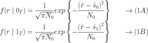
Assume that the BPSK symbols are transmitted through an AWGN channel characterized by variance = N0/2 Watts. When 0 is transmitted, the received symbol is represented by a Gaussian random variable ‘r‘ with mean=S0 = and variance =N0/2. When 1 is transmitted, the received symbol is represented by a Gaussian random variable – r with mean=S1= and variance =N0/2. Hence the conditional density function of the BPSK symbol (Figure 2) is given by,
Figure 1: BPSK – ideal constellation
Figure 2: Probability density function (PDF) for BPSK Symbols
An optimum receiver for BPSK can be implemented using a correlation receiver or a matched filter receiver (Figure 3). Both these forms of implementations contain a decision making block that decides upon the bit/symbol that was transmitted based on the observed bits/symbols at its input.
Figure 3: Optimum Receiver for BPSK
When the BPSK symbols are transmitted over an AWGN channel, the symbols appears smeared/distorted in the constellation depending on the SNR condition of the channel. A matched filter or that was previously used to construct the BPSK symbols at the transmitter. This process of projection is illustrated in Figure 4. Since the assumed channel is of Gaussian nature, the continuous density function of the projected bits will follow a Gaussian distribution. This is illustrated in Figure 5.
Figure 4: Role of correlation/Matched Filter
After the signal points are projected on the basis function axis, a decision maker/comparator acts on those projected bits and decides on the fate of those bits based on the threshold set. For a BPSK receiver, if the a-prior probabilities of transmitted 0’s and 1’s are equal (P=0.5), then the decision boundary or threshold will pass through the origin. If the apriori probabilities are not equal, then the optimum threshold boundary will shift away from the origin.
Figure 5: Distribution of received symbols
Considering a binary symmetric channel, where the apriori probabilities of 0’s and 1’s are equal, the decision threshold can be conveniently set to T=0. The comparator, decides whether the projected symbols are falling in region A or region B (see Figure 4). If the symbols fall in region A, then it will decide that 1 was transmitted. It they fall in region B, the decision will be in favor of ‘0’.
For deriving the performance of the receiver, the decision process made by the comparator is applied to the underlying distribution model (Figure 5). The symbols projected on the axis will follow a Gaussian distribution. The threshold for decision is set to T=0. A received bit is in error, if the transmitted bit is ‘0’ & the decision output is ‘1’ and if the transmitted bit is ‘1’ & the decision output is ‘0’.
This is expressed in terms of probability of error as,
Or equivalently,
By applying Bayes Theorem↗, the above equation is expressed in terms of conditional probabilities as given below,
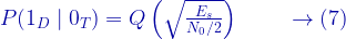
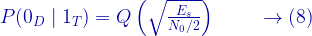
Since a-prior probabilities are equal P(0T)= P(1T) =0.5, the equation can be re-written as
Intuitively, the integrals represent the area of shaded curves as shown in Figure 6. From the previous article, we know that the area of the shaded region is given by Q function.
Figure 6a, 6b: Calculating Error Probability
Similarly,
From (4), (6), (7) and (8),
For BPSK, since Es=Eb, the probability of symbol error (Ps) and the probability of bit error (Pb) are same. Therefore, expressing the Ps and Pb in terms of Q function and also in terms of complementary error function :
Rate this article: Note: There is a rating embedded within this post, please visit this post to rate it.
This website uses cookies to improve your experience while you navigate through the website. Out of these, the cookies that are categorized as necessary are stored on your browser as they are essential for the working of basic functionalities of the website. We also use third-party cookies that help us analyze and understand how you use this website. These cookies will be stored in your browser only with your consent. You also have the option to opt-out of these cookies. But opting out of some of these cookies may affect your browsing experience.
Necessary cookies are absolutely essential for the website to function properly. These cookies ensure basic functionalities and security features of the website, anonymously.
Cookie
Duration
Description
cookielawinfo-checbox-analytics
11 months
This cookie is set by GDPR Cookie Consent plugin. The cookie is used to store the user consent for the cookies in the category "Analytics".
cookielawinfo-checbox-analytics
11 months
This cookie is set by GDPR Cookie Consent plugin. The cookie is used to store the user consent for the cookies in the category "Analytics".
cookielawinfo-checbox-functional
11 months
The cookie is set by GDPR cookie consent to record the user consent for the cookies in the category "Functional".
cookielawinfo-checbox-functional
11 months
The cookie is set by GDPR cookie consent to record the user consent for the cookies in the category "Functional".
cookielawinfo-checbox-others
11 months
This cookie is set by GDPR Cookie Consent plugin. The cookie is used to store the user consent for the cookies in the category "Other.
cookielawinfo-checbox-others
11 months
This cookie is set by GDPR Cookie Consent plugin. The cookie is used to store the user consent for the cookies in the category "Other.
cookielawinfo-checkbox-necessary
11 months
This cookie is set by GDPR Cookie Consent plugin. The cookies is used to store the user consent for the cookies in the category "Necessary".
cookielawinfo-checkbox-performance
11 months
This cookie is set by GDPR Cookie Consent plugin. The cookie is used to store the user consent for the cookies in the category "Performance".
viewed_cookie_policy
11 months
The cookie is set by the GDPR Cookie Consent plugin and is used to store whether or not user has consented to the use of cookies. It does not store any personal data.
Functional cookies help to perform certain functionalities like sharing the content of the website on social media platforms, collect feedbacks, and other third-party features.
Performance cookies are used to understand and analyze the key performance indexes of the website which helps in delivering a better user experience for the visitors.
Analytical cookies are used to understand how visitors interact with the website. These cookies help provide information on metrics the number of visitors, bounce rate, traffic source, etc.


![f_X(x) = \frac{1}{ \sqrt{ 2 \pi \sigma^2 }} exp \left[ -\frac{ \left( x-\mu \right) ^2}{2 \sigma^2} \right]](https://s0.wp.com/latex.php?latex=f_X%28x%29+%3D+%5Cfrac%7B1%7D%7B+%5Csqrt%7B+2+%5Cpi+%5Csigma%5E2+%7D%7D+exp+%5Cleft%5B+-%5Cfrac%7B+%5Cleft%28+x-%5Cmu+%5Cright%29+%5E2%7D%7B2+%5Csigma%5E2%7D+%5Cright%5D+&bg=ffffff&fg=000&s=2&c=20201002)