Mathuranathan Viswanathan, is an author @ gaussianwaves.com that has garnered worldwide readership. He is a masters in communication engineering and has 12 years of technical expertise in channel modeling and has worked in various technologies ranging from read channel, OFDM, MIMO, 3GPP PHY layer, Data Science & Machine learning.
Additionally, 5G NR supports π/2-BPSK in uplink (to be combined with OFDM with CP or DFT-s OFDM with CP)[1][2]. Utilization of π/2-BPSK in the uplink is aimed at providing further reduction of peak-to-average power ratio (PAPR) and boosting RF amplifier power efficiency at lower data-rates.
π/2 BPSK
π/2 BPSK uses two sets of BPSK constellations that are shifted by 90°. The constellation sets are selected depending on the position of the bits in the input sequence. Figure (1) depicts the two constellation sets for π/2 BPSK that are defined as per equation (1)
b[i] = input bits; i = position or index of input bits; d[i] = mapped bits (constellation points)
Figure 1: Two rotated constellation sets for use in π/2 BPSK
Equation (2) is for conventional BPSK – given for comparison. Figure (2) and Figure (3) depicts the ideal constellations and waveforms for BPSK and π/2 BPSK, when a long sequence of random input bits are input to the BPSK and π/2 BPSK modulators respectively. From the waveform, you may note that π/2 BPSK has more phase transitions than BPSK. Therefore π/2 BPSK also helps in better synchronization, especially for cases with long runs of 1s and 0s in the input sequence.
Key focus: Array pattern multiplication: total radiation pattern of N identical antennas is product of single-antenna radiation vector and array factor.
An antenna array is a collection of numerous linked antenna elements that operate together to broadcast or receive radio waves as if they were a single antenna. Phased array antennas are used to focus the radiated power towards a particular direction. The angular pattern of the phased array depends on the number of antenna elements, their geometrical arrangement in the array, and relative amplitudes and phases of the array elements.
Phased array antennas can be used to steer the radiated beam towards a particular direction by adjusting the relative phases of the array elements.
The basic property of antenna arrays is the translational phase-shift.
Time-shift property of Fourier transform
Let’s focus for a moment on the time-shifting property of Fourier transform. The time–shifting property implies that a shift in time corresponds to a phase rotation in the frequency domain.
Now, let’s turn our attention to antenna elements translated/shift in space. Figure 1 depicts a single antenna element having current density J(r) placed at the origin is moved in space to a new location that is l0 distant from the original position. The current density of the antenna element at the new position l0 is given by
\[J_{l_0}(r) = J(r – l_0) \quad \quad (2)\]
Figure 1: Current density of antenna element shifted in space
Therefore, from equations (2) and (3), the radiation vector of the antenna element space-shifted to new position l0 is given by the space shift property (similar to time-shift property of Fourier transform in equation (1))
\[\begin{aligned} \mathbf{F}_{l_0} \left(\mathbf{k} \right) &=\int_V J_{l_0}(r)e^{j \mathbf{k} \cdot r } d^3 r \\
&= \int_V J(r-l_0)e^{j \mathbf{k} \cdot r } d^3 r \\ &= \int_V J(r)e^{j \mathbf{k} \cdot (r+l_0) } d^3 r \\
&= e^{j \mathbf{k} l_0}\int_V J(r)e^{j \mathbf{k} \cdot r } d^3 r \\ &= e^{j \mathbf{k} l_0} \mathbf{F} \left(\mathbf{k} \right) \end{aligned}
\\
\Rightarrow \boxed{ \mathbf{F}_{l_0} \left(\mathbf{k} \right) = e^{j \mathbf{k} l_0} \mathbf{F}\left(\mathbf{k} \right) }
\quad \quad (4) \]
Note: The sign of exponential in the Fourier transform does not matter (it just indicates phase rotation in opposite direction), as long as the same convention is used throughout the analysis.
From equation (4), we can conclude that the relative location of the antenna elements with regard to one another causes relative phase changes in the radiation vectors, which can then contribute constructively in certain directions or destructively in others.
Array factor and array pattern multiplication
Figure 2 depicts a more generic case of identical antenna elements placed in three dimensional space at various radial distances l0, l1, l2, l3, … and the antenna feed coefficients respectively are a0, a1, a2, a3,…
Figure 2: Current densities of antenna elements shifted in space – contributors to array factor of phased array antenna
The current densities of the individual antenna elements are
The quantity A(k) is called array factor which incorporates the relative translational phase shifts and the relative feed coefficients of the array elements.
The array pattern multiplication property states that the total radiation pattern of an antenna array constructed with N identical antennas is the product of radiation vector of a single individual antenna element (also called as element factor) and the array factor.
Effect of array factor on power gain and radiation intensity
Let U(θ,ɸ) and G(θ,ɸ) denote the radiation intensity and the power gain patterns of an antenna element. The total radiation intensity and the power gain of an antenna array, constructed with such identical antenna elements, will be modified by the array factor as follows.
The role of array factor is very similar to that of the transfer function of an linear time invariant system. Recall that if a wide sense stationary process x(t) is input to the LTI system defined by the transfer function H(f), then the power spectral density of the output is given by
\[S_y(f) = \mid H(f) \mid ^2 S_x(f)\]
Illustration using a linear array of half-wave dipole antennas
Linear antennas are electrically thin antennas whose conductor diameter is very small compared to the wavelength of the radiation λ.
A linear antenna oriented along the z-axis has radiation vector (field) whose components are along the directions of the radial distance and the polar angle. That is, the radiation intensity U(θ,ɸ) and the power gain G(θ,ɸ) depend only on the polar angle θ. In other words, the radiation intensity and the power gain are omnidirectional (independent of azimuthal angle ɸ).
Figure 3, illustrates an antenna array with linear half-wave dipoles placed on the x-axis at equidistant from each other.
Figure 3: A linear antenna array with half-wave dipole elements
We are interested in the power gain pattern G(θ,ɸ) of the antenna array shown in Figure 3.
The normalized power gain pattern of an individual antenna element (half-wave dipole) is given by
Figure 4 illustrates equation (15) – the effect of array factor on normalized power gain of an array of half-wave dipole antennas. The plot is generated for separation distance between antenna elements l=λ and the feed coefficients for the antenna elements a = [1, -1, 1].
Check out my Google colab for the python code. The results are given below.
Figure 4: Illustrating the effect of array pattern multiplication on normalized power gain of antenna array
Key focus: Far-field region is dominated by radiating terms of antenna fields, hence, knowing the far field retarded potentials is of interest.
Introduction
The fundamental premise of understanding antenna radiation is to understand how a radiation source influences the propagation of travelling electromagnetic waves. Propagation of travelling waves is best described by electric and magnetic potentials along the propagation path.
The concept of retarded potentials was introduced in this post.
The electromagnetic field travels at certain velocity and hence the potentials at the observation point (due to the changing charge at source) are experienced after a certain time delay. Such potentials are called retarded potentials.
The retarded potentials at a radial distance r from an antenna source fed with a single frequency sinusoidal waves, is shown to be
\[\begin{aligned} \Phi(r) &= \frac{1}{4 \pi \epsilon} \int_V \frac{\rho(z')e^{-j k R }}{R} d^3 z' \\ A(r) &= \frac{\mu}{4 \pi} \int_V \frac{J(z')e^{-j k R }}{R} d^3 z' \end{aligned} \quad \quad (1)\]
where, the quantity k = ω/c = 2 π/λ is called the free-space wavenumber. Also, ρ is the charge density, J is the current density, Φ is the electric potential and A is the magnetic potential that are functions of both radial distance.
Far-field region
Figure 1 illustrates the two scenarios: (a) the receiver is ‘nearer’ to the antenna source (b) the receiver is ‘far away’ from the antenna source.
Figure 1: Radiation fields when antenna and receiver are (a) near and (b) far away
Since the far-field region is dominated by radiating terms of the antenna fields, we are interested in knowing the retarded potentials in the far-field region. The far field region is shown to be
\[\frac{2 l^2}{ \lambda} < r < \infty \quad \quad (2)\]
where l is the length of the antenna element and λ is the wavelength of the signal from the antenna.
Figure 2: Spherical coordinate system on a cartesian coordinate system
Antenna radiation patterns are generally visualized in a spherical coordinate system (Figure (2)). In a coordinate system, each unit vector can be expressed as the cross product of other two unit vectors. Hence,
We note that the term inside the integral is dependent on polar angle (θ) and azimuthal angle (ɸ). It determines the directional properties of the radiation. The term outside the integral is dependent on radial distance r. These terms can be expressed separately
The terms that determine the directional properties: Q(θ,ɸ) & F(θ,ɸ) are called charge form-factor and radiation vector respectively. The charge form-factor Q(θ,ɸ) and the radiation vector F(θ,ɸ) are three dimensional spatial Fourier transforms of charge density ρ(z’) and current density J(z) respectively.
We are in the process of building antenna models. In that journey, we started with the fundamental Maxwell’s equations in electromagnetism, then looked at retarded potentials that are solutions for Maxwell’s equations. Propagation of travelling waves is best described by retarded potentials along the propagation path. Then, the boundary between near-field and far-field regions was defined. Since most of the antenna radiation analysis are focused in the far-field regions, we looked at retarded potentials in the far-field region.
Rate this article: Note: There is a rating embedded within this post, please visit this post to rate it.
Antennas are radiation sources of finite physical dimension. To a distant observer, the radiation waves from the antenna source appears more like a spherical wave and the antenna appears to be a point source regardless of its true shape. The terms far-field and near-field are associated with such observations/antenna measurement. The terms imply that there must exist a boundary between the near field and far field.
Essentially, the near field and far field are regions around an antenna source. Though the boundary between these two regions are not fixed in space, the antenna measurements made in these regions differ significantly. One method of establishing the boundary between the near-field and far-field regions is to look at the acceptable level of phase error in the antenna measurements.
An antenna designer is interested in studying how the phase of the radiation waves launched from the antenna source is affected by the distance between the antenna source and the receiver (observation point). As the distance between the antenna and the receiver increases, there exists a phase difference between the measurements taken along the two lines shown. This phase difference contribute to antenna measurement errors, it also affects retarded potentials and radiation fields.
Near-field and far-field approximations
Figure 1 illustrates the two scenarios: (a) the receiver is ‘nearer’ to the antenna source (b) the receiver is ‘far away’ from the antenna source. The antenna is of standard dimension of length l. The figures show two rays – one from the origin to the observation point P (on the yz plane) and the other from the mid-point of distance z’=l/2 from the origin towards the observation point P.
In Figure(2)(b), the observation point P is at a distance that is very far from the antenna source element. The term ‘far’ implies that the distance r is much greater than the spatial extent of the current distribution of the antenna element, that is, r >> z’. Also, the two rays appear parallel to each other.
Figure 1: Radiation fields when antenna and receiver are (a) near and (b) far away
The essence of the following exercise is to determine the boundary between the ‘near’ and the ‘far’ field regions of the antenna. Once that boundary is established, we can determine whether far field approximation can be used on the antenna measurements or for the calculation of retarded potentials/fields produced by the antenna.
\[\begin{aligned} \Phi(r) &= \frac{1}{4 \pi \epsilon} \int_V \frac{\rho(z')e^{-j k R }}{R} d^3 z' \quad\quad (1) \\ A(r) &= \frac{\mu}{4 \pi} \int_V \frac{J(z')e^{-j k R }}{R} d^3 z' \quad\quad (2) \end{aligned}\]
We note that we cannot arbitrarily set R=r, because any small relative difference between R and r, will result in phase errors in the retarded potentials such that e-j k R ≠ e-j k r . Solving for the relationship between R and r is the crux of the radiation boundary problem.
From Figure (1)(a), applying law of cosines, the distance R can be written as
\[R = \sqrt{r^2 – 2 r z' cos \theta + z'^2} \quad \quad (3)\]
which can be expanded using the following Binomial series expansion,
On the other hand, from Figure (1)(b), the distance \(R\) is given by
\[R = r – z’ cos \theta \quad \quad (6)\]
As r → ∞, equation (4) approaches exactly the parallel ray approximation given by equation (6). However, for finite values of r (due to the additional term z’ 2/2r sin2 θ and also the additional terms that were neglected) there exists an error between parallel ray approximation and the actual value of R computed using equation (4).
So the question is: What is the minimum distance over which the parallel ray approximation can be invoked ?
According to text books, for the maximum extent of the antenna (z’ = l/2), when the maximum phase difference is π/8, it produces acceptable errors in antenna measurements.
In these equations, k = ω/c = 2 π/ λ is the free-space wavenumber.
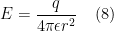
Equation (8) defines the minimum distance (a.k.a the boundary between near and far field regions) over which the parallel ray approximation can be invoked. This minimum distance is called far-field distance – the boundary beyond which the far-field region starts. The quantity l is the maximum dimension of the antenna.
The far-field region, also known as Fraunhofer region, is dominated by radiating terms of the antenna fields. The far-field region is
\[\boxed{\frac{2 l^2}{ \lambda} < r < \infty }\quad \quad (9)\]
Figure 2: Far-field distance and far-field region
Rate this article: Note: There is a rating embedded within this post, please visit this post to rate it.
Key focus: Understand retarded potentials – the basic building block for understanding antenna array patterns. Retarded potentials are potentials at an observation point when the quantities at the source are non-static (varies in both space and time)
The static case : potentials
The fundamental premise of understanding antenna radiation is to understand how a radiation source influences the propagation of travelling electromagnetic waves. Propagation of travelling waves are best described by electric and magnetic potentials along the propagation path.
In the static case, the electric field E, charge density ρ, current density J and the electric potential Φ , magnetic field B and magnetic potential A are all constant in time. That is, they are functions of radial distance r in the spherical co-ordinate system, but not functions of time t . The solution for Maxwell’s equations (in the spherical co-ordinate system) take the following equivalent form in terms of electric and magnetic potentials:
Figure 1: Potentials – solutions for Maxwell’s equations for static case
The quantity R is the distance between the source and the point at which the corresponding fields are observed and d3 r’ is the volume element at the source point.
The non-static case : retarded potentials
Since electromagnetic radiation are produced by time-varying electric charges, we are interested in describing the potentials at a given the observation point for this non-static situation. Obviously for the non-static case, the electric field E , charge density ρ , current density J and the electric potential Φ , magnetic field B and magnetic potential A are functions of both radial distance and time. The corresponding formulas for the potentials are
With c defined as the velocity of light, the factor t – R/c is the time delay between the emission of electromagnetic photon from the source and the time it gets observed by an observer. The electromagnetic field travels at certain velocity and hence the potentials at the observation point (due to the changing charge at source) are experienced after a certain time delay. Such potentials are called retarded potentials and the propagation delay t – R/c is called retarded time. Hence, we can say that the retarded potentials are related to electromagnetic fields of a current or charge distribution that vary in time.
Figure 2: Retarded potentials – solutions for Maxwell’s equations for non-static case
Sinusoidal time dependence of retarded potentials
In antenna theory, the antenna elements (source) are fed with sinusoidal waves. So, the next step is to express the retarded potentials at the observation point when all the quantities at source vary sinusoidally in time. Therefore, when the quantities are sinusoidal single-frequency waves, the shift property of Fourier transform can be applied.
The retarded potential A(r,t) can be derived in a similar manner. Therefore, the retarded potentials (equations (3) and (4) ) for the single frequency sinusoidal wave is given by
\[\boxed{ \begin{aligned} \Phi(r) &= \frac{1}{4 \pi \epsilon} \int_V \frac{\rho(r')e^{-j k R }}{R} d^3 r' \\ A(r) &= \frac{\mu}{4 \pi} \int_V \frac{J(r')e^{-j k R }}{R} d^3 r' \end{aligned} }\]
In these equations, the quantity k = ω/c = 2 π/λ is called the free-space wavenumber.
Rate this article: Note: There is a rating embedded within this post, please visit this post to rate it.
Key focus: Briefly look at the building blocks of antenna array theory starting from the fundamental Maxwell’s equations in electromagnetism.
Maxwell’s equations
Maxwell’s equations are a collection of equations that describe the behavior of electromagnetic fields. The equations relate the electric fields () and magnetic fields () to their respective sources – charge density () and current density ( ).
Maxwell’s equations are available in two forms: differential form and integral form. The integral forms of Maxwell’s equations are helpful in their understanding the physical significance.
Maxwell’s equation (1):
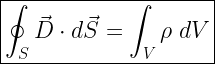
The flux of the displacement electric field through a closed surface equals the total electric charge enclosed in the corresponding volume space .
This is also called Gauss law for electricity.
Consider a point charge +q in a three dimensional space. Assuming a symmetric field around the charge and at a distance r from the charge, the surface area of the sphere is .
Figure 1: Illustration of Coulomb’s law using Maxwell’s equation
Therefore, left side of the equation is simply equal to the surface area of the sphere multiplied by the magnitude of the electric displacement vector .
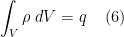
For the right hand side of the Maxwell’s equation (1), the integral of the charge density over a volume V is simply equal to the charge enclosed. Therefore,
The electric displacement field is a measure of electric field in the material after taking into account the effect of the material on the electric field. The electric field and the displacement field are related by the permittivity of the material as
Combining equations (5), (6) and (7), yields the magnitude of an electric field as derived from Coulomb’s law
Maxwell’s equation (2)
The flux of the magnetic field through a closed surface is zero. That is, the net of magnetic field that “flows into” and “flows out of” a closed surface is zero.
This implies that there are no source or sink for the magnetic flux lines, in other words – they are closed field lines with no beginning or end. This is also called Gauss law for magnetic field.
Figure 2: Gauss law for magnetic field
Maxwell’s equation (3)
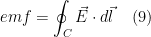
The work done on an electric charge as it travels around a closed loop conductor is the electromotive force (emf). Therefore, the left side of the gives the emf induced in a circuit.
The right side of the equation is the rate of change of magnetic flux through the circuit.
Hence, the Maxwell’s third equation is actually the Faraday’s (and Len’s) law of magnetic induction
The electromotive force (emf) induced in a circuit is directly proportional to the rate of change of magnetic flux through the circuit.
Figure 3: Faraday’s law for magnetic induction
Maxwell’s equation (4)
The circulating magnetic field is denoted by the circulation of magnetizing field around a closed curved path : . The electric current is denoted by the flux of current density () through any surface spanning that curved path. The quantity denotes the rate of change of displacement current through any surface spanning that curved path.
According to Maxwell’s extension to the Ampere’s law , magnetic fields can be generated in two ways: with electric current and with changing electric flux. The equation states that the electric current or change in electric flux through a surface produces a circulating magnetic field around any path that bounds that surface.
Summary of Maxwell’s equations
The electric field leaving a volume space is proportional to the electric charge contained in the volume.
The net of magnetic field that “flows into” and “flows out of” a closed surface is zero. There is no concept called magnetic charge/magnetic monopole.
A changing magnetic flux through a circuit induces electromotive force in the circuit
Magnetic fields are produced by electric current as well as by changing electric flux.
Rate this article: Note: There is a rating embedded within this post, please visit this post to rate it.
Key focus: Briefly look at linear antennas and various dipole antennas and plot the normalized power gain pattern in polar plot and three dimensional plot.
Linear antennas
Linear antennas are electrically thin antennas whose conductor diameter is very small compared to the wavelength of the radiation λ.
Viewed in a spherical coordinate system (Figure 1), for linear antenna, the antenna is oriented along the z-axis such that the radiation vector has only components along directions of the radial distance Fr and the polar angle Fθ. The radiation vector is determined by the current density J which is characterized by the current distribution I(z)[1].
Figure 1: Electrical and magnetic fields from a current source
Figure 2: Linear antenna element
Hertzian dipole (infinitesimally small dipole)
Hertzian dipole is the simplest configuration of a linear antenna used for study purposes. It is an infinitesimally small (typically [2]) antenna element that has the following current density distribution
\[I(z) = I \; L\; \delta(z)\]
The radiation vector Fz (θ) is given by [1]
\[F_z(\theta) = \int_{-L/2}^{L/2} I(z^{'}) e^{jk_z z^{'}} dz{'} = \int_{-L/2}^{L/2} I L \delta(z{'}) e^{jkz{'}cos \theta} dz{'} = IL\]
The normalized power gain of the Hertzian dipole is [2]
\[g(\theta) = C_0 sin^{2} \theta \]
where, C0 is a constant chosen to make maximum of g(θ) equal to unity and θ is the polar angle in the spherical coordinate system.
Center-fed dipole (standing wave antenna)
For the center-fed small dipole antenna, the current distribution is assumed to be a standing wave. Defining k = 2π/λ as the wave number and h = L/2 as the half-length of the antenna, the current distribution and the normalized power gain g(θ) are given by
\[I(z) = I \; sin \left[ k \left(L/2 – |z| \right) \right]\]
\[g(\theta) =C_n \left|\frac{cos (k h \; cos \theta) – cos( k h) }{sin \theta} \right| ^2\]
where, Cn is a constant chosen to make maximum of g(θ) equal to unity and θ is the polar angle in the spherical coordinate system.
Figure 3: Center-fed small dipole
For half-wave dipole, set L = λ/2 or kl = π. Therefore, the current distribution for half-wave dipole shrinks to
Let’s plot the normalized power gain pattern of Hertzian & Half-wave dipole antennas in polar plot and three dimensional plot.
Check out my Google colab for the python code to plot the normalized power gain in polar plot as well as three dimensional plot. The results are given below.
Figure 4: Hertzian dipole – power gain pattern (polar plot)
Figure 5: Hertzian dipole – power gain pattern (3D plot)
Figure 6: Half-wave dipole – power gain pattern (polar plot)
Figure 7: Half-wave dipole power gain 3d plot (cartesian coordinates)
Figure 8: Normalized power gain pattern for dipole of length
Figure 9: Normalized power gain pattern for dipole of length (3D projection)
Rate this article: Note: There is a rating embedded within this post, please visit this post to rate it.
Key focus: Bayes’ theorem is a method for revising the prior probability for specific event, taking into account the evidence available about the event.
Introduction
In statistics, the process of drawing conclusions from data subject to random variations – is called “statistical inference”. Usually, in any random experiment, the observations are recorded and conclusions have to be drawn based on the recorded data set. Conclusions over the underlying random process are necessary to establish one or many of the following:
* Estimation of a parameter of interest (For example: the carrier frequency estimation in the receiver) * Confidence and credibility of the estimate * Rejecting a preconceived hypothesis * Classification of data set into groups
Several schools of statistical inference have evolved over time. Bayesian inference is one of them.
Bayes’ theorem
Bayes’ theorem is central to scientific discovery and a core tool in machine learning/AI. It has numerous applications including but not limited to areas such as: mathematics, medicine, finance, marketing and engineering.
The Bayes’ theorem is used in Bayesian inference, usually dealing with a sequence of events, as new information becomes available about a subsequent event, that new information is used to update the probability of the initial event. In this context, we encounter two flavors of probabilities: prior probability and posterior probability.
Prior probability : This is the initial probability about an event before any information is available about the event. In other words, this is the initial belief about a particular hypothesis before any evidence is available about the hypothesis.
Posterior probability: This is the probability value that has been revised by using new information that is later obtained from a subsequent event. In other words, this is the updated belief about the hypothesis as new evident becomes available.
The formula for Bayes’ theorem is
Figure 1: Formula for Bayes’ theorem
A very simple thought experiment
You are asked to conduct a random experiment with a given coin. You are told that the coin is unbiased (probability of obtaining head or tail is equal and is exactly 50%). You believe (before conducting the experiment) that the coin is unbiased and that the chance of getting head or tail is equal to be 0.5.
Assume that you have not looked at both sides of the coin and simply you start to conduct the experiment. You start to toss the coin repeatedly and record the events (This is the observed new information/evidences). On the first toss you observe the coin lands on the ground with head faced up. On the second toss, again the head shows up. On subsequent tosses, the coin always shows up head. You have tossed 100 times and all these tosses you observe only head. Now what will you think about the coin? You will really start to think that both sides of the coin are engraved with “head” (no tail etched on the coin). Now, based on the new evidences, your belief about the “unbiasedness” of the coin is altered.
This is what Bayes’ theorem or Bayesian inference is all about. It is a general principle about learning from experience. It connects beliefs (called prior probabilities) and evidences (observed data). Based on the evidence, the degree of belief is refined. The degree of belief after conducting the experiment is called posterior probability.
Figure 2: Bayes’ theorem – the process
Real world example
Suppose, a person X falls sick and goes to the doctor for diagnosis. The doctor runs a series of tests and the test result came positive for a rare disease that affects 0.1% of the population. The accuracy of the test is 99%. That is, the test can correctly identify 99% of people that have the disease and will incorrectly report disease in only 1% of the people that do not have the disease. Now, how certain is that the person X actually have the disease ?
In this scenario, we can apply the extended form of Bayes’ theorem
Figure 3: Bayes’ theorem – extended form
Extended form of Bayes’ theorem is applied in special scenarios where P(H) is a binary variable, which implies it can take only two possible states. In the given problem above, the hypothesis can take only two states – H – “having the disease” and H̅ – “not having the disease”.
For the given problem, we can come up with the following numbers for the various quantities in the extended form of Bayes’ theorem.
P(H) = prior probability of having the disease before the availability of test results. This is often guess work, but luckily we have the probability that affects the population (0.1% = 0.001) to replace this. P(E/H) = probability to test positive for the disease if person X has the disease (99% = 0.99) P(H̅) = probability of NOT having the disease (1-0.001 = 0.999) P(E/H̅) = probability of NOT having the disease and falsely identified positive by the test (1% = 0.01). P(H/E) = probability of person X actually have the disease given the test result is positive.
Plugging-in these numbers in the extended form of Bayes’ theorem, we get the probability that X actually have the disease is just 9%.
Figure 4: Calculation using extended form of Bayes’ theorem
Person X doubts the result and goes for a second opinion to another doctor and gets tested from an independent laboratory. The second test result came back positive this time too. Now what is the probability that person X actually have the disease ?
P(H) = Replace this with the posterior probability from first test (we are refining the belief about the result of the first test) = 9.016% = 0.09016 P(E/H) = probability to test positive for the disease if person X has the disease (99% = 0.99) P(H̅) = probability of NOT having the disease from first test (1-0.09016 = 0.90984) P(E/H̅) = probability of NOT having the disease and falsely identified positive by the second test (1% = 0.01). P(H/E) = probability of person X actually have the disease given the second test result is also positive.
Figure 5: Refining the belief about the first test using results from second test
Therefore, the updated probability based on two positive tests is 90.75%. This implies that there is a 90.75% chance that person X has the disease.
I hope the reader got a better understanding of what Bayes’ theorem is, various parameters in the equation for Bayes’ theorem and how to apply it.
Rate this article: Note: There is a rating embedded within this post, please visit this post to rate it.
Line code is the signaling scheme used to represent data on a communication line. There are several possible mapping schemes available for this purpose. Lets understand and demonstrate line code and PSD (power spectral density) in Matlab & Python.
Line codes – requirements
When transmitting binary data over long distances encoding the binary data using line codes should satisfying following requirements.
All possible binary sequences can be transmitted.
The line code encoded signal must occupy small transmission bandwidth, so that more information can be transmitted per unit bandwidth.
Error probability of the encoded signal should be as small as possible
Since long distance communication channels cannot transport low frequency content (example : DC component of the signal , such line codes should eliminate DC when encoding). The power spectral density of the encoded signal should also be suitable for the medium of transport.
The receiver should be able to extract timing information from the transmitted signal.
Guarantee transition of bits for timing recovery with long runs of 1s and 0s in the binary data.
Support error detection and correction capability to the communication system.
Unipolar Non-Return-to-Zero (NRZ) level and Return-to-Zero (RZ) level codes
Unipolar NRZ(L) is the simplest of all the line codes, where a positive voltage represent binary bit 1 and zero volts represents bit 0. It is also called on-off keying.
In unipolar return-to-zero (RZ) level line code, the signal value returns to zero between each pulse.
Unipolar Non Return to Zero (NRZ) and Return to Zero (RZ) line code – 5V peak voltage
For both unipolar NRZ and RZ line coded signal, the average value of the signal is not zero and hence they have a significant DC component (note the impulse at zero frequency in the power spectral density (PSD) plot).
The DC impulses in the PSD do not carry any information and it also causes the transmission wires to heat up. This is a wastage of communication resource.
Unipolar coded signals do not include timing information, therefore long runs of 0s and 1s can cause loss of synchronization at the receiver.
Power spectral density of unipolar NRZ line code
Power spectral density of unipolar RZ line code
Bipolar Non-Return-to-Zero (NRZ) level code
In bipolar NRZ(L) coding, binary bit 1 is mapped to positive voltage and bit 0 is mapped to negative voltage. Since there are two opposite voltages (positive and negative) it is a bipolar signaling scheme.
Bipolar Non Return to Zero (NRZ) and Return to Zero (RZ) line code – 5V peak voltage
Evident from the power spectral densities, the bipolar NRZ signal is devoid of a significant impulse at the zero frequency (DC component is very close to zero). Furthermore, it has more power than the unipolar line code (note: PSD curve for bipolar NRZ is slightly higher compared to that of unipolar NRZ). Therefore, bipolar NRZ signals provide better signal-to-noise ratio (SNR) at the receiver.
Bipolar NRZ signal lacks embedded clock information, which posses synchronization problems at the receiver when the binary information has long runs of 0s and 1s.
Comparing power spectral densities of bipolar NRZ and unipolar NRZ line codes
Alternate Mark Inversion (AMI)
AMI is a bipolar signaling method, that encodes binary 0 as 0 Volt and binary 1 as +ve and -ve voltage (alternating between successive 1s).
Alternate Mark Inversion (AMI) line code – 5V peak voltage
AMI eliminates DC component. Evident from the PSD plots below, AMI has reduced bandwidth (narrower bumps) and faster roll-offs compared to unipolar and bipolar NRZ line codes.
It has inbuilt error detection mechanism: a bit error results in violation of bipolar signaling. It has guaranteed timing transitions even for long runs of 1s and 0s.
Power spectral density of Alternate Mark Inversion (AMI) compared with unipolar and bipolar NRZ line codes
Manchester encoding
In Manchester encoding, the signal for each binary bit contains one transition. For example, bit 0 is represented by a transition from negative to positive voltage and bit 1 is represented by transitioning from one positive to negative voltage. Therefore, it is considered to be self clocking and it is devoid of DC component.
Digitally Manchester encoding can be implemented by XORing the binary data and the clock, followed by mapping the output to appropriate voltage levels.
Manchester encoding
From the PSD plot, we can conclude that Manchester encoded signal occupies twice the bandwidth of Bipolar NRZ(L) encoded signal.
Power spectral density of Manchester encoding compared with that of Bipolar NRZ(L)
Matlab script
In this script, lines codes are simulated and their power spectral density (PSD) are plotted using pwelch command.
%Simulate line codes and plot power spectral densities (PSD)
%Author: Mathuranathan Viswanathan
clearvars; clc;
L = 32; %number of digital samples per data bit
Fs = 8*L; %Sampling frequency
voltageLevel = 5; %peak voltage level in Volts
data = rand(10000,1)>0.5; %random 1s and 0s for data
clk = mod(0:2*numel(data)-1,2).'; %clock samples

ami = 1*data; previousOne = 0; %AMI encoding
for ii=1:numel(data)
    if (ami(ii)==1) && (previousOne==0)
        ami(ii)= voltageLevel;
        previousOne=1;
    end
    if (ami(ii)==1) && (previousOne==1)
        ami(ii)= -voltageLevel;
        previousOne = 0;
    end
end

%converting the bits to sequences and mapping to voltage levels
clk_sequence=reshape(repmat(clk,1,L).',1,length(clk)*L);
data_sequence=reshape(repmat(data,1,2*L).',1,length(data)*2*L);
unipolar_nrz_l = voltageLevel*data_sequence;
nrz_encoded = voltageLevel*(2*data_sequence - 1);
unipolar_rz = voltageLevel*and(data_sequence,not(clk_sequence));
ami_sequence = reshape(repmat(ami,1,2*L).',1,length(ami)*2*L);
manchester_encoded = voltageLevel*(2*xor(data_sequence,clk_sequence)-1);

figure; %Plot signals in time domain
subplot(7,1,1); plot(clk_sequence(1:800)); title('Clock');
subplot(7,1,2); plot(data_sequence(1:800)); title('Data')
subplot(7,1,3); plot(unipolar_nrz_l(1:800)); title('Unipolar non-return-to-zero level')
subplot(7,1,4); plot(nrz_encoded(1:800)); title('Bipolar Non-return-to-zero level')
subplot(7,1,5); plot(unipolar_rz(1:800)); title('Unipolar return-to-zero')
subplot(7,1,6); plot(ami_sequence(1:800)); title('Alternate Mark Inversion (AMI)')
subplot(7,1,7); plot(manchester_encoded(1:800)); title('Manchester Encoded - IEEE 802.3')

figure; %Plot power spectral density
ns = max(size(unipolar_nrz_l));
na = 16;%averaging factor to plot averaged welch spectrum
w = hanning(floor(ns/na));%Hanning window
%Plot Welch power spectrum using Hanning window
[Pxx1,F1] = pwelch(unipolar_nrz_l,w,[],[],1,'onesided');
[Pxx2,F2] = pwelch(nrz_encoded,w,[],[],1,'onesided');
[Pxx3,F3] = pwelch(unipolar_rz,w,[],[],1,'onesided');
[Pxx4,F4] = pwelch(ami_sequence,w,[],[],1,'onesided'); %
[Pxx5,F5] = pwelch(manchester_encoded,w,[],[],1,'onesided');

semilogy(F1,Pxx1,'DisplayName','Unipolar-NRZ-L');hold on;
semilogy(F2,Pxx2,'DisplayName','Bipolar NRZ(L)');
semilogy(F3,Pxx3,'DisplayName','Unipolar-RZ');
semilogy(F4,Pxx4,'DisplayName','AMI');
semilogy(F5,Pxx5,'DisplayName','Manchester');
legend();
Key focus: Euclidean & Hamming distances are used to measure similarity or dissimilarity between two sequences. Used in Soft & Hard decision decoding.
Distance is a measure that indicates either similarity or dissimilarity between two words. Given a pair of words a=(a0,a1, … ,an-1) and b=(b0,b1,…,bn-1) , there are variety of ways one can characterize the distance, d(a,b), between the two words. Euclidean and Hamming distances are familiar ones. Euclidean distance is extensively applied in analysis of convolutional codes and Trellis codes. Hamming distance is frequently encountered in the analysis of block codes.
In contrast to classical hard-decision decoders (see below) which operate on binary values, a soft-decision decoder directly processes the unquantized (or quantized in more than two levels in practice) samples at the output of the matched filter for each bit-period, thereby avoiding the loss of information.
If the outputs of the matched filter at each bit-period are unquantized or quantized in more than two levels, the demodulator is said to make soft-decisions. The process of decoding the soft-decision received sequence is called soft-decision decoding. Since the decoder uses the additional information contained in the multi-level quantized or unquantized received sequence, soft-decision decoding provides better performance compared to hard-decision decoding. For soft-decision decoding, metrics like likelihood function, Euclidean distance and correlation are used.
For illustration purposes, we consider the communication system model shown in Figure 1. A block encoder encodes the information blocks m=(m1,m2,…,mk) and generates the corresponding codeword vector c=(c1,c2,…,cn). The codewords are modulated and sent across an AWGN channel. The received signal is passed through a matched filter and the multi-level quantizer outputs the soft-decision vector r .
Figure 1: Soft-decision receiver model for decoding linear block codes for AWGN channel
The goal of a decoder is to produce an estimate m̂ of the information sequence m based on the received sequence r. Equivalently, the information sequence m and the codeword c has one-to-one correspondence, the decoder can also produce an estimate ĉ of the codeword c. If the codeword c was transmitted, a decoding error occurs if ĉ ≠ c.
For equi-probable codewords, The decoder that selects a codeword that maximizes the conditional probability P(r, c). This is called a maximum lihelihood decoder (MLD).
For an AWGN channel with two-sided power spectral density N0/2, the conditional probability is given by
The sum is the squared Euclidean distance between the received sequence r and the coded signal sequence s. We can note that the term is common for all codewords and n is a constant. This simplifies the MLD decoding rule where we select a codeword from the code dictionary that minimizes the Euclidean distance D(r, s)$.
Hamming distance
Hamming distance between two words a=(a0,a1, … ,an-1) and b=(b0,b1,…,bn-1) in Galois FieldGF(2), is the number of coordinates in which the two blocks differ.
For example, the Hamming distance between (0,0,0,1) and (1,0,1,0) in GF(2) is 3, since they differ in three digits. For an independent and identically distributed (i.i.d) error model with (discrete) uniform error amplitude distribution, the most appropriate measure is Hamming distance.
Minimum distance
The minimum distance of block code C, is the smallest distance between all distance pairs of code words in C. The minimum distance of a block code determines both its error-detecting ability and error-correcting ability. A large minimum distance guarantees reliability against random errors. The general relationship between a block code’s minimum distance and the error-detecting and error correcting capability is as follows.
● If dmin is the minimum Hamming distance of a block code, the code is guaranteed to detect up to e=dmin-1 errors. Consequently, let c1 and c2 be the two closest codewords in the codeword dictionary C. If c1 was transmitted and c2 is received, the error is undetectable.
● If dmin is the minimum Hamming distance of a block code and if the optimal decoding procedure of nearest-neighbor decoding is used at the receiver, the code is guaranteed to correct up to t=(dmin-1 )/2 errors.
Sub-optimal hard decision decoding
In soft-decision decoding, the bit samples to the decoder are eitherunquantized or quantized to multi-levels and the maximum likelihood decoder (MLD) needs to compute M correlation metrics, where M is the number of codewords in the codeword dictionary. Although this provides the best performance, the computational complexity of the decoder increases when the number of codewords M becomes large. To reduce the computational burden, the output of the matched filter at each bit-period can be quantized to only two levels, denoted as 0 and 1, that results in a hard-decision binary sequence. Then, the decoder processes this hard-decision sequence based on a specific decoding algorithm. This type of decoding, illustrated in Figure 1, is called hard-decision decoding.
Figure 2: Hard-decision receiver model for decoding linear block codes for AWGN channel
The hard-decision decoding methods use Hamming distance metric to decode the hard-decision received sequence to the closest codeword. The objective of such decoding methods is to choose a codeword that provides the minimum Hamming distance with respect to the hard-decision received sequence. Since the hard-decision samples are only quantized to two levels, resulting in loss of information, the hard-decision decoding results in performance degradation when compared to soft-decision decoding.
Decoding using standard array and syndrome decoding are popular hard-decision decoding methods encountered in practice.
Rate this article: Note: There is a rating embedded within this post, please visit this post to rate it.
This website uses cookies to improve your experience while you navigate through the website. Out of these, the cookies that are categorized as necessary are stored on your browser as they are essential for the working of basic functionalities of the website. We also use third-party cookies that help us analyze and understand how you use this website. These cookies will be stored in your browser only with your consent. You also have the option to opt-out of these cookies. But opting out of some of these cookies may affect your browsing experience.
Necessary cookies are absolutely essential for the website to function properly. These cookies ensure basic functionalities and security features of the website, anonymously.
Cookie
Duration
Description
cookielawinfo-checbox-analytics
11 months
This cookie is set by GDPR Cookie Consent plugin. The cookie is used to store the user consent for the cookies in the category "Analytics".
cookielawinfo-checbox-analytics
11 months
This cookie is set by GDPR Cookie Consent plugin. The cookie is used to store the user consent for the cookies in the category "Analytics".
cookielawinfo-checbox-functional
11 months
The cookie is set by GDPR cookie consent to record the user consent for the cookies in the category "Functional".
cookielawinfo-checbox-functional
11 months
The cookie is set by GDPR cookie consent to record the user consent for the cookies in the category "Functional".
cookielawinfo-checbox-others
11 months
This cookie is set by GDPR Cookie Consent plugin. The cookie is used to store the user consent for the cookies in the category "Other.
cookielawinfo-checbox-others
11 months
This cookie is set by GDPR Cookie Consent plugin. The cookie is used to store the user consent for the cookies in the category "Other.
cookielawinfo-checkbox-necessary
11 months
This cookie is set by GDPR Cookie Consent plugin. The cookies is used to store the user consent for the cookies in the category "Necessary".
cookielawinfo-checkbox-performance
11 months
This cookie is set by GDPR Cookie Consent plugin. The cookie is used to store the user consent for the cookies in the category "Performance".
viewed_cookie_policy
11 months
The cookie is set by the GDPR Cookie Consent plugin and is used to store whether or not user has consented to the use of cookies. It does not store any personal data.
Functional cookies help to perform certain functionalities like sharing the content of the website on social media platforms, collect feedbacks, and other third-party features.
Performance cookies are used to understand and analyze the key performance indexes of the website which helps in delivering a better user experience for the visitors.
Analytical cookies are used to understand how visitors interact with the website. These cookies help provide information on metrics the number of visitors, bounce rate, traffic source, etc.