Mathuranathan, Author at GaussianWaves

Fading channel – complex baseband equivalent models

Keyfocus: Fading channel models for simulation. Learn how fading channels can be modeled as FIR filters for simplified modulation & detection. Rayleigh/Rician fading.

Introduction

A fading channel is a wireless communication channel in which the quality of the signal fluctuates over time due to changes in the transmission environment. These changes can be caused by different factors such as distance, obstacles, and interference, resulting in attenuation and phase shifting. The signal fluctuations can cause errors or loss of information during transmission.

Fading channels are categorized into slow fading and fast fading depending on the rate of channel variation. Slow fading occurs over long periods, while fast fading happens rapidly over short periods, typically due to multipath interference.

To overcome the negative effects of fading, various techniques are used, including diversity techniques, equalization, and channel coding.

Fading channel in frequency domain

With respect to the frequency domain characteristics, the fading channels can be classified into frequency selective and frequency-flat fading.

A frequency flat fading channel is a wireless communication channel where the attenuation and phase shift of the signal are constant across the entire frequency band. This means that the signal experiences the same amount of fading at all frequencies, and there is no frequency-dependent distortion of the signal.

In contrast, a frequency selective fading channel is a wireless communication channel where the attenuation and phase shift of the signal vary with frequency. This means that the signal experiences different levels of fading at different frequencies, resulting in a frequency-dependent distortion of the signal.

Frequency selective fading can occur due to various factors such as multipath interference and the presence of objects that scatter or absorb certain frequencies more than others. To mitigate the effects of frequency selective fading, various techniques can be used, such as equalization and frequency hopping.

The channel fading can be modeled with different statistics like Rayleigh, Rician, Nakagami fading. The fading channel models, in this section, are utilized for obtaining the simulated performance of various modulations over Rayleigh flat fading and Rician flat fading channels. Modeling of frequency selective fading channel is discussed in this article.

Linear time invariant channel model and FIR filters

The most significant feature of a real world channel is that the channel does not immediately respond to the input. Physically, this indicates some sort of inertia built into the channel/medium, that takes some time to respond. As a consequence, it may introduce distortion effects like inter-symbol interference (ISI) at the channel output. Such effects are best studied with the linear time invariant (LTI) channel model, given in Figure 1.

*Figure 1: Complex baseband equivalent LTI channel model*

Linear time invariant channel model for simulating fading channels — *Figure 1: Complex baseband equivalent LTI channel model*

In this model, the channel response to any input depends only on the channel impulse response(CIR) function of the channel. The CIR is usually defined for finite length \(L\) as \(\mathbf{h}=[h_0,h_1,h_2, \cdots,h_{L-1}]\) where \(h_0\) is the CIR at symbol sampling instant \(0T_{sym}\) and \(h_{L-1}\) is the CIR at symbol sampling instant \((L-1)T_{sym}\). Such a channel can be modeled as a tapped delay line (TDL) filter, otherwise called finite impulse response (FIR) filter. Here, we only consider the CIR at symbol sampling instances. It is well known that the output of such a channel (\(\mathbf{r}\)) is given as the linear convolution of the input symbols (\(\mathbf{s}\)) and the CIR (\(\mathbf{h}\)) at symbol sampling instances. In addition, channel noise in the form of AWGN can also be included the model. Therefore, the resulting vector of from the entire channel model is given as

\[\mathbf{r} = \mathbf{h} \ast \mathbf{s} +\mathbf{n} \quad\quad (1) \]

This article is part of the following books
● Digital Modulations using Matlab : Build Simulation Models from Scratch, ISBN: 978-1521493885
● Digital Modulations using Python ISBN: 978-1712321638
● Wireless communication systems in Matlab ISBN: 979-8648350779
All books available in ebook (PDF) and Paperback formats

Simulation model for detection in flat fading channel

A flat-fading (also called as frequency-non-selective) channel is modeled with a single tap (\(L=1\)) FIR filter with the tap weights drawn from distributions like Rayleigh, Rician or Nakagami distributions. We will assume block fading, which implies that the fading process is approximately constant for a given transmission interval. For block fading, the random tap coefficient \(h=h[0]\) is a complex random variable (not random processes) and for each channel realization, a new set of complex random values are drawn from Rayleigh or Rician or Nakagami fading according to the type of fading desired.

*Figure 2: LTI channel viewed as tapped delay line filter*

Simulation models for modulation and detection over a fading channel is shown in Figure 2. For a flat fading channel, the output of the channel can be expressed simply as the product of time varying channel response and the input signal. Thus, equation (1) can be simplified (refer this article for derivation) as follows for the flat fading channel.

\[\mathbf{r} = h\mathbf{s} + \mathbf{n} \quad\quad (2) \]

Since the channel and noise are modeled as a complex vectors, the detection of \(\mathbf{s}\) from the received signal is an estimation problem in the complex vector space.

*Figure 3: Simulation model for modulation and detection over flat fading channel*

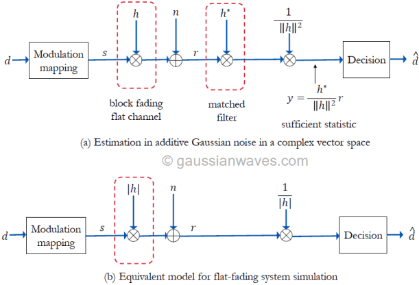
Assuming perfect channel knowledge at the receiver and coherent detection, the receiver shown in Figure 3(a) performs matched filtering. The impulse response of the matched filter is matched to the impulse response of the flat-fading channel as \( h^{\ast}\). The output of the matched filter is scaled down by a factor of \(||h||^2\) which is the total-energy contained in the impulse response of the flat-fading channel. The resulting decision vector \(\mathbf{y}\) serves as the sufficient statistic for the estimation of \(\mathbf{s}\) from the received signal \(\mathbf{r}\) (refer equation A.77 in reference [1])

\[\tilde{\mathbf{y}} = \frac{h^{\ast}}{||h||^2} \mathbf{r} = \frac{h^{\ast}}{||h||^2} h\mathbf{s} + \frac{h^{\ast}}{||h||^2} \mathbf{n} = \mathbf{s} + \tilde{\mathbf{w}} \quad\quad (3) \]

Since the absolute value \(|h|\) and the Eucliden norm \(||h||\) are related as \(|h|^2= \left\lVert h\right\rVert = hh^{\ast}\), the model can be simplified further as given in Figure 3(b).

To simulate flat fading, the values for the fading variable \(h\) are drawn from complex normal distribution

\[h= X + jY \quad\quad (4) \]

where, \(X,Y\) are statistically independent real valued normal random variables.

● If \(E[h]=0\), then \(|h|\) is Rayleigh distributed, resulting in a Rayleigh flat fading channel
● If \(E[h] \neq 0\), then \(|h|\) is Rician distributed, resulting in a Rician flat fading channel with the factor \(K=[E[h]]^2/\sigma^2_h\)

References

[1] D. Tse and P. Viswanath, Fundamentals of Wireless Communication, Cambridge University Press, 2005.↗

Books by the author

Wireless Communication Systems in Matlab Second Edition(PDF) Note: There is a rating embedded within this post, please visit this post to rate it. Checkout Added to cart	Digital Modulations using Python (PDF ebook) Note: There is a rating embedded within this post, please visit this post to rate it. Checkout Added to cart	Digital Modulations using Matlab (PDF ebook) Note: There is a rating embedded within this post, please visit this post to rate it. Checkout Added to cart
Hand-picked Best books on Communication Engineering Best books on Signal Processing

Central Limit Theorem – a demonstration

Central Limit Theorem – What is it ?

The central limit theorem (CLT) is a fundamental concept in statistics and probability theory that explains how the sum of independent and identically distributed random variables behaves. The theorem states that as the number of these variables increases, the distribution of their sum tends to become more like a normal distribution, even if the variables themselves are not normally distributed.

CLT states that the sum of independent and identically distributed (i.i.d) random variables (with finite mean and variance) approaches normal distribution as sample size \(N \rightarrow \infty\). In simpler terms, the theorem states that under certain general conditions, the sum of independent observations that follow same underlying distribution approximates to normal distribution. The approximation steadily improves as the number of observations increase. The underlying distribution of the independent observation can be anything – binomial, Poisson, exponential, Chi-Squared etc.

Why CLT ?

CLT is an important concept in statistics because it allows us to make inferences about a population based on a sample, even if we do not know the distribution of the population. It is used in many statistical techniques, such as hypothesis testing and confidence intervals.

Applications of CLT

Central limit theorem (CLT) is applied in a vast range of applications including (but not limited to) signal processing, channel modeling, random process, population statistics, engineering research, predicting the confidence intervals, hypothesis testing, etc. One such application in signal processing is – deriving the response of a cascaded series of low pass filters by applying the CLT. In the article titled ‘the central limit theorem and low-pass filters‘ the author has illustrated how the response of a cascaded series of low pass filters approaches Gaussian shape as the number of filters in the series increase [1].

In digital communication, the effect of noise on a communication channel is modeled as additive Gaussian white noise. This follows from the fact that the noise from many physical channels can be considered approximately Gaussian. For example, the random movement of electrons in the semiconductor devices gives rise to shot noise whose effect can be approximated to Gaussian distribution by applying central limit theorem.

Law of large numbers and CLT

there is a connection between the central limit theorem and the law of large numbers.

The law of large numbers is another important theorem in probability theory, which states that as the number of independent and identically distributed (iid) random variables increases, the average of those variables converges to the expected value of the distribution. In other words, as the sample size increases, the sample mean becomes more and more representative of the true population mean.

The central limit theorem, on the other hand, describes the distribution of the sum of iid random variables, and shows that as the sample size increases, the distribution of the sum approaches a normal distribution.

Both the law of large numbers and the CLT deal with the behavior of the sum or average of iid random variables as the sample size gets larger. The law of large numbers describes the behavior of the sample mean, while the CLT describes the behavior of the sum of the variables.

In essence, the law of large numbers is a precursor to the central limit theorem, as it establishes the fact that the sample mean becomes more and more representative of the true population mean as the sample size increases, and the central limit theorem shows that the distribution of the sum of iid random variables approaches a normal distribution as the sample size gets larger.

Demonstration using Python

For Matlab code, please refer the following book – Wireless communication systems in Matlab – by Mathuranathan Viswanathan

The following Python code illustrate how the theorem comes to play when the number of observations is increased for two separate experiments: rolling \(N\) unbiased dice and tossing \(N\) unbiased coins. The code generates \(N\) i.i.d discrete uniform random variables that generates uniform random numbers from the set \(\left\{1,k\right\}\). In the case of the dice rolling experiment, \(k\) is set to \(6\), thus simulating the random pick from the sample space \(S=\left\{1,2,3,4,5,6\right\}\) with equal probability. For the coin tossing experiment, \(k\) is set to \(2\), thus simulating the sample space of \(S=\left\{1,2\right\}\) representing head or tail events with equal probability. Rest of the code is self explanatory.

Python code

#---------Central limit theorem - Author: Mathuranathan #gaussianwaves.com -----------------------
#
import numpy as np
import matplotlib.pyplot as plt
#%matplotlib inline

numIterations = np.asarray([1,2,5,10,50,100]); #number of i.i.d RVs
experiment = 'dice' #valid values: 'dice', 'coins'
maxNumForExperiment = {'dice':6,'coins':2} #max numbers represented on dice or coins
nSamp=100000

k = maxNumForExperiment[experiment]

fig, fig_axes = plt.subplots(ncols=3, nrows=2, constrained_layout=True)

for i,N in enumerate(numIterations):
    y = np.random.randint(low=1,high=k+1,size=(N,nSamp)).sum(axis=0)
    row = i//3;col=i%3;
    bins=np.arange(start=min(y),stop=max(y)+2,step=1)
    fig_axes[row,col].hist(y,bins=bins,density=True)
    fig_axes[row,col].set_title('N={} {}'.format(N,experiment))
plt.show()

***Figure 1: Demonstrating central limit theorem using N numbers of dice***

***Figure 2: Demonstrating central limit theorem using N numbers of coins***

References

[1] Engelberg, “The central limit theorem and low-pass filters”, Proceedings of the 2004 11th IEEE International Conference on Electronics, Circuits and Systems, 13-15 Dec. 2004, pp. 65-68.↗

Books by the author

Wireless Communication Systems in Matlab Second Edition(PDF) Note: There is a rating embedded within this post, please visit this post to rate it. Checkout Added to cart	Digital Modulations using Python (PDF ebook) Note: There is a rating embedded within this post, please visit this post to rate it. Checkout Added to cart	Digital Modulations using Matlab (PDF ebook) Note: There is a rating embedded within this post, please visit this post to rate it. Checkout Added to cart
Hand-picked Best books on Communication Engineering Best books on Signal Processing

Maximum Likelihood estimation

Keywords: maximum likelihood estimation, statistical method, probability distribution, MLE, models, practical applications, finance, economics, natural sciences.

Introduction

Maximum Likelihood Estimation (MLE) is a statistical method used to estimate the parameters of a probability distribution by finding the set of values that maximize the likelihood function of the observed data. In other words, MLE is a method of finding the most likely values of the unknown parameters that would have generated the observed data.

The likelihood function is a function that describes the probability of observing the data given the parameters of the probability distribution. The MLE method seeks to find the set of parameter values that maximizes this likelihood function.

For example, suppose we have a set of data that we believe to be normally distributed, but we do not know the mean or variance of the distribution. We can use MLE to estimate these parameters by finding the mean and variance that maximize the likelihood function of the observed data.

The MLE method is widely used in statistical inference, hypothesis testing, and model fitting in many areas, including economics, finance, engineering, and the natural sciences. MLE is a powerful and flexible method that can be applied to a wide range of statistical models, making it a valuable tool in data analysis and modeling.

Difference between MLE and MLD

Maximum likelihood estimation (MLE) and maximum likelihood decoding (MLD) are two different concepts used in different contexts.

Maximum likelihood estimation is a statistical method used to estimate the parameters of a probability distribution based on a set of observed data. The goal is to find the set of parameter values that maximize the likelihood function of the observed data. MLE is commonly used in statistical inference, hypothesis testing, and model fitting.

On the other hand, maximum likelihood decoding (MLD) is a method used in digital communications and signal processing to decode a received signal that has been transmitted through a noisy channel. The goal is to find the transmitted message that is most likely to have produced the received signal, based on a given probabilistic model of the channel.

In maximum likelihood decoding, the receiver calculates the likelihood of each possible transmitted message, given the received signal and the channel model. The maximum likelihood decoder then selects the transmitted message that has the highest likelihood as the decoded message.

While both MLE and MLD involve the concept of maximum likelihood, they are used in different contexts. MLE is used in statistical estimation, while MLD is used in digital communications and signal processing for decoding.

MLE applied to communication systems

Maximum Likelihood estimation (MLE) is an important tool in determining the actual probabilities of the assumed model of communication.

In reality, a communication channel can be quite complex and a model becomes necessary to simplify calculations at decoder side.The model should closely approximate the complex communication channel. There exist a myriad of standard statistical models that can be employed for this task; Gaussian, Binomial, Exponential, Geometric, Poisson,etc., A standard communication model is chosen based on empirical data.

Each model mentioned above has unique parameters that characterizes them. Determination of these parameters for the chosen model is necessary to make them closely model the communication channel at hand.

Suppose a binomial model is chosen (based on observation of data) for the error events over a particular channel, it is essential to determine the probability of succcess (\(p\)) of the binomial model.

If a Gaussian model (normal distribution!!!) is chosen for a particular channel then estimating mean (\(\mu\)) and variance (\(\sigma^{2}\)) are necessary so that they can be applied while computing the conditional probability of p(y received | x sent)

Similarly estimating the mean number of events within a given interval of time or space (\(\lambda\)) is a necessity for a Poisson distribution model.

Maximum likelihood estimation is a method to determine these unknown parameters associated with the corresponding chosen models of the communication channel.

Python code example for MLE

The following program is an implementation of maximum likelihood estimation (MLE) for the binary symmetric channel (BSC) using the binomial probability mass function (PMF).

The goal of MLE is to estimate the value of an unknown parameter (in this case, the error probability \(p\)) based on observed data. The BSC is a simple channel model where each transmitted bit is flipped (with probability \(p\)) independently of other bits during transmission. The goal of the following program is to estimate the error probability \(p\) of the BSC based on a given binary data sequence.

import numpy as np
from scipy.optimize import minimize
from scipy.special import binom
import matplotlib.pyplot as plt

def BSC_MLE(data):
    """
    Maximum likelihood estimation (MLE) for the Binary Symmetric Channel (BSC).
    This function estimates the error probability p of the BSC based on the observed data.
    """
    
    # Define the binomial probability mass function
    def binom_PMF(p):
        n = len(data)
        k = np.sum(data)
        p = np.clip(p, 1e-10, 1 - 1e-10)  # Regularization to avoid problems due to small estimation errors
        logprob = np.log(binom(n, k)) + k*np.log(p) + (n-k)*np.log(1-p)
        return -logprob
    
    # Use the minimize function from scipy.optimize to find the value of p that maximizes the binomial PMF
    #x0 argument specifies the initial guess for the value of p that maximizes the binomial PMF. For BSC x0=0.5
    #BFGS is Broyden-Fletcher-Goldfarb-Shanno optimization algorithm used for unconstrained nonlinear optimization
    res = minimize(lambda p: binom_PMF(p), x0=0.5, method='BFGS')
    p_est = res.x[0]

    # Plot the observed data as a histogram
    plt.hist(data, bins=2, density=True, alpha=0.5)
    plt.axvline(p_est, color='r', linestyle='--')
    plt.xlabel('Bit value')
    plt.ylabel('Frequency')
    plt.title('Observed data')
    plt.show()
    
    return p_est

data = np.random.randint(2, size=1000)
p_est = BSC_MLE(data)
print('Estimated error probability: {:.4f}'.format(p_est))

The program first defines a function called BSC_MLE that takes a binary data sequence as input and returns the estimated error probability p_est. The BSC_MLE function defines the binomial PMF, which represents the probability of observing a certain number of errors (i.e., bit flips) in the data sequence given a specific error probability p. The binomial PMF is then maximized using the minimize function from the scipy.optimize module to find the value of p that maximizes the likelihood of observing the data.

The program then generates a random binary data sequence of length 100 using the np.random.randint() function and calls the BSC_MLE function to estimate the error probability based on the observed data. Finally, the program prints the estimated error probability. Try increasing the sequence length to 1000 and observe the estimated error probability.

***Figure 1: Maximum Likelihood Estimation (MLE) : Plotting the observed data as a histogram***

Reference :

[1] – Maximum Likelihood Estimation – a detailed explanation by S.Purcell

Books by the author

Wireless Communication Systems in Matlab Second Edition(PDF) Note: There is a rating embedded within this post, please visit this post to rate it. Checkout Added to cart	Digital Modulations using Python (PDF ebook) Note: There is a rating embedded within this post, please visit this post to rate it. Checkout Added to cart	Digital Modulations using Matlab (PDF ebook) Note: There is a rating embedded within this post, please visit this post to rate it. Checkout Added to cart
Hand-picked Best books on Communication Engineering Best books on Signal Processing

Maximum Likelihood Decoding

Keywords: maximum likelihood decoding, digital communication, data storage, noise, interference, wireless communication systems, optical communication systems, digital storage systems, probability, likelihood estimation, python

Introduction

Maximum likelihood decoding is a technique used to determine the most likely transmitted message in a digital communication system, based on the received signal and statistical models of noise and interference. The method uses maximum likelihood estimation to calculate the probability of each possible transmitted message and then selects the one with the highest probability.

To perform maximum likelihood decoding, the receiver uses a set of pre-defined models to estimate the likelihood of each possible transmitted message based on the received signal. The method is commonly used in various digital communication and data storage systems, such as wireless communication and digital storage. However, it can be complex and time-consuming, particularly in systems with large message spaces or complex noise and interference models.

Maximum Likelihood Decoding:

Consider a set of possible codewords (valid codewords – set \(Y\)) generated by an encoder in the transmitter side. We pick one codeword out of this set ( call it \(y\) ) and transmit it via a Binary Symmetric Channel (BSC) with probability of error \(p\) ( To know what is a BSC – click here ). At the receiver side we receive the distorted version of \(y\) ( call this erroneous codeword \(x\)).

Maximum Likelihood Decoding chooses one codeword from \(Y\) (the list of all possible codewords) which maximizes the following probability.

\[\mathbb{P}(y\;sent\mid x\;received )\]

Meaning that the receiver computes \(P(y_1,x) , P(y_2,x) , P(y_3,x),\cdots,P(y_n,x)\). and chooses a codeword (\(y\)) which gives the maximum probability. In practice we don’t know \(y\) (at the receiver) but we know \(x\). So how to compute the probability ? Maximum Likelihood Estimation (MLE) comes to our rescue. For a detailed explanation on MLE – refer here^[1] The aim of maximum likelihood estimation is to find the parameter value(s) that makes the observed data most likely. Understanding the difference between prediction and estimation is important at this point. Estimation differs from prediction in the following way … In estimation problems, likelihood of the parameters is estimated based on given data/observation vector. In prediction problems, probability is used as a measure to predict the outcome from known parameters of a model.

Examples for “Prediction” and “Estimation” :

1) Probability of getting a “Head” in a single toss of a fair coin is \(0.5\). The coin is tossed 100 times in a row.Prediction helps in predicting the outcome ( head or tail ) of the \(101^{th}\) toss based on the probability.

2) A coin is tossed 100 times and the data ( head or tail information) is recorded. Assuming the event follows Binomial distribution model, estimation helps in determining the probability of the event. The actual probability may or may not be \(0.5\). Maximum Likelihood Estimation estimates the conditional probability based on the observed data ( received data – \(x\)) and an assumed model.

Example of Maximum Likelihood Decoding:

Let \(y=11001001\) and \(x=10011001\) . Assuming Binomial distribution model for the event with probability of error \(0.1\) (i.e the reliability of the BSC is \(1-p = 0.9\)), the Hamming distance between codewords is \(2\) . For binomial model,

\[\mathbb{P}(y\;received\mid x\;sent ) = (1-p)^{n-d}.p^{d}\]

where \(d\) =the hamming distance between the received and the sent codewords n= number of bit sent
\(p\)= error probability of the BSC.
\(1-p\) = reliability of BSC

Substituting \(d=2, n=8\) and \(p=0.1\) , then \(P(y\;received \mid x\;sent) = 0.005314\).

Note : Here, Hamming distance is used to compute the probability. So the decoding can be called as “minimum distance decoding” (which minimizes the Hamming distance) or “maximum likelihood decoding”. Euclidean distance may also be used to compute the conditional probability.

As mentioned earlier, in practice \(y\) is not known at the receiver. Lets see how to estimate \(P(y \;received \mid x\; sent)\) when \(y\) is unknown based on the binomial model.

Since the receiver is unaware of the particular \(y\) corresponding to the \(x\) received, the receiver computes \(P(y\; received \mid x\; sent)\) for each codeword in \(Y\). The \(y\) which gives the maximum probability is concluded as the codeword that was sent.

Python code implementing Maximum Likelihood Decoding:

The following program for demonstrating the maximum likelihood decoding, involves generating a noisy signal from a transmitted message and then using maximum likelihood decoding to estimate the transmitted message from the noisy signal.

The maximum_likelihood_decoding function takes three arguments: received_signal, noise_variance, and message_space.
The calculate_probabilities function is called to calculate the probability of each possible message given the received signal, using the known noise variance.
The probabilities are normalized so that they sum to 1.
The maximum_likelihood_decoding function finds the index of the most likely message (i.e., the message with the highest probability).
The function returns the most likely message.
An example usage is demonstrated where a binary message space is defined ([0, 1]), along with a noise variance and a transmitted message.
The transmitted message is added to noise to generate a noisy received signal.
The maximum_likelihood_decoding function is called to decode the noisy signal.
The transmitted message, received signal, and decoded message are printed to the console for evaluation.

import numpy as np
import matplotlib.pyplot as plt

# Define a function to calculate the probability of each possible message given the received signal
def calculate_probabilities(received_signal, noise_variance, message_space):
    probabilities = np.zeros(len(message_space))

    for i, message in enumerate(message_space):
        error = received_signal - message
        probabilities[i] = np.exp(-np.sum(error ** 2) / (2 * noise_variance))

    return probabilities / np.sum(probabilities)

# Define a function to perform maximum likelihood decoding
def maximum_likelihood_decoding(received_signal, noise_variance, message_space):
    probabilities = calculate_probabilities(received_signal, noise_variance, message_space)
    most_likely_message_index = np.argmax(probabilities)
    return message_space[most_likely_message_index]

# Example usage
message_space = np.array([0, 1])
noise_variance = 0.4
transmitted_message = 1
received_signal = transmitted_message + np.sqrt(noise_variance) * np.random.randn()
decoded_message = maximum_likelihood_decoding(received_signal, noise_variance, message_space)

print('Transmitted message:', transmitted_message)
print('Received signal:', received_signal)
print('Decoded message:', decoded_message)

# Plot probability distribution
probabilities = calculate_probabilities(received_signal, noise_variance, message_space)
plt.bar(message_space, probabilities)
plt.title('Probability Distribution for Received Signal = {}'.format(received_signal))
plt.xlabel('Transmitted Message')
plt.ylabel('Probability')
plt.ylim([0, 1])
plt.show()

The probability of the received signal given a specific transmitted message is calculated as follows:

Compute the difference between the received signal and the transmitted message.
Compute the sum of squares of this difference vector.
Divide this sum by twice the known noise variance.
Take the negative exponential of this value.

This results in a probability density function (PDF) for the received signal given the transmitted message, assuming that the noise is Gaussian and zero-mean.

The probabilities for each possible transmitted message are then normalized so that they sum to 1. This is done by dividing each individual probability by the sum of all probabilities.

The maximum_likelihood_decoding function determines the most likely transmitted message by selecting the message with the highest probability, which corresponds to the maximum likelihood estimate of the transmitted message given the received signal and the statistical model of the noise.

Sample outputs

Transmitted message: 1
Received signal: 0.21798306949364643
Decoded message: 0

Transmitted message: 1
Received signal: -0.5115453787966966
Decoded message: 0

Transmitted message: 1
Received signal: 0.8343088336355061
Decoded message: 1

Transmitted message: 1
Received signal: -0.5479891887158619
Decoded message: 0

The probability distribution for the last sample output is shown below

Figure: Probability distribution for a sample run of the code

Reference :

[1] – Maximum Likelihood Estimation – a detailed explanation by S.Purcell

Books by the author

Wireless Communication Systems in Matlab Second Edition(PDF) Note: There is a rating embedded within this post, please visit this post to rate it. Checkout Added to cart	Digital Modulations using Python (PDF ebook) Note: There is a rating embedded within this post, please visit this post to rate it. Checkout Added to cart	Digital Modulations using Matlab (PDF ebook) Note: There is a rating embedded within this post, please visit this post to rate it. Checkout Added to cart
Hand-picked Best books on Communication Engineering Best books on Signal Processing

Hard and Soft decision decoding

What are hard and soft decision decoding

Hard decision decoding and soft decision decoding are two different methods used for decoding error-correcting codes.

With hard decision decoding, the received signal is compared to a set threshold value to determine whether the transmitted bit is a 0 or a 1. This is commonly used in digital communication systems that experience noise or interference, resulting in a low signal-to-noise ratio.

Soft decision decoding, on the other hand, treats the received signal as a probability distribution and calculates the likelihood of each possible transmitted bit based on the characteristics of the received signal. This approach is often used in modern digital communication and data storage systems where the signal-to-noise ratio is relatively high and there is a need for higher accuracy and reliability.

While soft decision decoding can achieve better error correction, it is more complex and computationally expensive than hard decision decoding.

More details

Let’s expatiate on the concepts of hard decision and soft decision decoding. Consider a simple even parity encoder given below.

Input Bit 1	Input Bit 2	Parity bit added by encoder	Codeword Generated
0	0	0	000
0	1	1	011
1	0	1	101
1	1	0	110

The set of all possible codewords generated by the encoder are 000,011,101 and 110.

Lets say we are want to transmit the message “01” through a communication channel.

Hard decision decoding

Case 1 : Assume that our communication model consists of a parity encoder, communication channel (attenuates the data randomly) and a hard decision decoder

The message bits “01” are applied to the parity encoder and we get “011” as the output codeword.

*Figure 1: Hard decision decoding – a simple illustration*

The output codeword “011” is transmitted through the channel. “0” is transmitted as “0 Volt and “1” as “1 Volt”. The channel attenuates the signal that is being transmitted and the receiver sees a distorted waveform ( “Red color waveform”). The hard decision decoder makes a decision based on the threshold voltage. In our case the threshold voltage is chosen as 0.5 Volt ( midway between “0” and “1” Volt ) . At each sampling instant in the receiver (as shown in the figure above) the hard decision detector determines the state of the bit to be “0” if the voltage level falls below the threshold and “1” if the voltage level is above the threshold. Therefore, the output of the hard decision block is “001”. Perhaps this “001” output is not a valid codeword ( compare this with the all possible codewords given in the table above) , which implies that the message bits cannot be recovered properly. The decoder compares the output of the hard decision block with the all possible codewords and computes the minimum Hamming distance for each case (as illustrated in the table below).

All possible Codewords	Hard decision output	Hamming distance
000	001	1
011	001	1
101	001	1
110	001	3

The decoder’s job is to choose a valid codeword which has the minimum Hamming distance. In our case, the minimum Hamming distance is “1” and there are 3 valid codewords with this distance. The decoder may choose any of the three possibility and the probability of getting the correct codeword (“001” – this is what we transmitted) is always 1/3. So when the hard decision decoding is employed the probability of recovering our data ( in this particular case) is 1/3. Lets see what “Soft decision decoding” offers …

Soft Decision Decoding

The difference between hard and soft decision decoder is as follows

In Hard decision decoding, the received codeword is compared with the all possible codewords and the codeword which gives the minimum Hamming distance is selected
In Soft decision decoding, the received codeword is compared with the all possible codewords and the codeword which gives the minimum Euclidean distance is selected. Thus the soft decision decoding improves the decision making process by supplying additional reliability information ( calculated Euclidean distance or calculated log-likelihood ratio)

For the same encoder and channel combination lets see the effect of replacing the hard decision block with a soft decision block.

*Figure 2: Soft-decision decoding – a simple illustration*

Voltage levels of the received signal at each sampling instant are shown in the figure. The soft decision block calculates the Euclidean distance between the received signal and the all possible codewords.

Valid codewords	Voltage levels at each sampling instant of received waveform	Euclidean distance calculation	Euclidean distance
0 0 0 ( 0V 0V 0V )	0.2V 0.4V 0.7V	(0-0.2)²+ (0-0.4)²+ (0-0.7)²	0.69
0 1 1 ( 0V 1V 1V )	0.2V 0.4V 0.7V	(0-0.2)²+ (1-0.4)²+ (1-0.7)²	0.49
1 0 1 ( 1V 0V 1V )	0.2V 0.4V 0.7V	(1-0.2)²+ (0-0.4)²+ (1-0.7)²	0.89
1 1 0 ( 1V 1V 0V )	0.2V 0.4V 0.7V	(1-0.2)²+ (1-0.4)²+ (0-0.7)²	1.49

The minimum Euclidean distance is “0.49” corresponding to “0 1 1” codeword (which is what we transmitted). The decoder selects this codeword as the output. Even though the parity encoder cannot correct errors, the soft decision scheme helped in recovering the data in this case. This fact delineates the improvement that will be seen when this soft decision scheme is used in combination with forward error correcting (FEC) schemes like convolution codes , LDPC etc

From this illustration we can understand that the soft decision decoders uses all of the information ( voltage levels in this case) in the process of decision making whereas the hard decision decoders does not fully utilize the information available in the received signal (evident from calculating Hamming distance just by comparing the signal level with the threshold whereby neglecting the actual voltage levels).

Note: This is just to illustrate the concept of Soft decision and Hard decision decoding. Prudent souls will be quick enough to find that the parity code example will fail for other voltage levels (e.g. : 0.2V , 0.4 V and 0.6V) . This is because the parity encoders are not capable of correcting errors but are capable of detecting single bit errors.

Soft decision decoding scheme is often realized using Viterbi decoders. Such decoders utilize Soft Output Viterbi Algorithm (SOVA) which takes into account the apriori probabilities of the input symbols producing a soft output indicating the reliability of the decision.

Rate this article: Note: There is a rating embedded within this post, please visit this post to rate it.

For further reading

[1] I. Dokmanic, R. Parhizkar, J. Ranieri and M. Vetterli, “Euclidean Distance Matrices: Essential theory, algorithms, and applications,” in IEEE Signal Processing Magazine, vol. 32, no. 6, pp. 12-30, Nov. 2015, doi: 10.1109/MSP.2015.2398954.↗

Books by the author

Wireless Communication Systems in Matlab Second Edition(PDF) Note: There is a rating embedded within this post, please visit this post to rate it. Checkout Added to cart	Digital Modulations using Python (PDF ebook) Note: There is a rating embedded within this post, please visit this post to rate it. Checkout Added to cart	Digital Modulations using Matlab (PDF ebook) Note: There is a rating embedded within this post, please visit this post to rate it. Checkout Added to cart
Hand-picked Best books on Communication Engineering Best books on Signal Processing

Matlab code for RS codes

Its been too long since I posted. For a kick start ,
i am continuing the theory on RS coding.
Here is a simple Matlab code (which can be found in Matlab Help, posted here with a little bit detailed explanation) for better understanding of RS code

%Matlab Code for RS coding and decoding

n=7; k=3; % Codeword and message word lengths
m=3; % Number of bits per symbol
msg = gf([5 2 3; 0 1 7;3 6 1],m) % Two k-symbol message words
% message vector is defined over a Galois field where the number must
%range from 0 to 2^m-1

codedMessage = rsenc(msg,n,k) % Two n-symbol codewords

dmin=n-k+1 % display dmin
t=(dmin-1)/2 % diplay error correcting capability of the code

% Generate noise – Add 2 contiguous symbol errors with first word;
% 2 discontiguous symbol errors with second word and 3 distributed symbol
% errors to last word
noise=gf([0 0 0 2 3 0 0 ;6 0 1 0 0 0 0 ;5 0 6 0 0 4 0],m)

received = noise+codedMessage

%dec contains the decoded message and cnumerr contains the number of
%symbols errors corrected for each row. Also if cnumerr(i) = -1 it indicates
%that the ith row contains unrecoverable error
[dec,cnumerr] = rsdec(received,n,k)
% print the original message for comparison
msg

% Given below is the output of the program. Only decoded message, cnumerr and original
% message are given here (with comments inline)

% The default primitive polynomial over which the GF is defined is D^3+D+1 ( which is 1011 -> 11 in decimal).

dec = GF(2^3) array. Primitive polynomial = D^3+D+1 (11 decimal)

Array elements =

5 2 3
0 1 7
6 6 7

cnumerr =

2
2
-1 ->>> Error in last row -> this error is due to the fact that we have added 3 distributed errors with the last row where as the RS code can correct only 2 errors. Compare the decoded message with original message given below for confirmation

% Original message printed for comparison
msg = GF(2^3) array. Primitive polynomial = D^3+D+1 (11 decimal)

Array elements =

5 2 3
0 1 7
3 6 1

Reference :
[1] Mathematics behind RS codes – Bernard Sklar – Click Here

Reed Solomon Codes – Introduction

The Hamming codes described in the previous articles are suitable for random bit errors in a sequence of transmitted bits. If the communication medium is prone to burst errors (channel errors affecting contiguous blocks of bits) (missing symbols are called erasures ), then Hamming code may not be suitable.

For example in CD, DVD and in Hard drives, the data is written in contiguous blocks and are retrieved in contiguous blocks. The heart of a hard disk is the read/write channel (an integral part of the disk drive controller SOC chip). The read/write channel is used to improve the signal to noise ratio of the data that is written into and read from the disk. Its design is aimed at providing reliable data retrieval from the disk. Algorithms like PRML (Partial Response signaling with Maximum Likelihood detection) are used to increase the areal densities of the disk (packing more bits in a given area on the disk platter). Error control coding is used to improve the performance of the detection algorithm and to protect the user data from erasures. In this case, a class of Error correcting codes called Reed Solomon Codes (RS Codes) are used. RS Codes have been utilized in hard disks for the past 15 to 20 years. RS codes are useful for channels having memory (like CD,DVD).

The other applications of RS Codes include:

1) Digital Subscriber line (DSL) and its variants like ADSL, VDSL…
2) Deep space and satellite communications
3) Barcodes
4) Digital Television
5) Microwave communication, Mobile communications and many more…

Reed Solomon Codes are linear block codes, a subset of the BCH codes called non-binary BCH. (n,k) RS code contains k data symbols and n-k parity symbols. RS Codes are also cyclic codes since the cyclic shift of any codeword will result in another valid RS codeword.

Note the usage of the word “symbols” instead of “bits” when referring to RS Codes. The word symbol is used to refer a group of bits. For example if I say that I am using a (7,3) RS Code with 5 bit symbols, it implies that each symbol is a collection of 5-bits and the RS Codeword is made up of 7 such symbols, of which 3 symbols represent data and remaining 4 symbols represent parity symbols.

A m-bit RS (n,k) Code can be defined using

where t is the symbol error correcting capability of the RS code. This code corrects t symbol errors. We can also see that the minimum distance for RS code is given by

This gives the maximum possible d_min. A code with maximum d_min is more reliable as it will be able to correct more errors.

Example:

Consider a (255,247) RS code , where each symbol is made up of m=8 bits. This code contains 255 symbols (each 8 bits of length) in a codeword of which 247 symbols are data symbols and the remaining 8 symbols are parity symbols. This code can correct any 4 symbol burst errors.

If the errors are not occurring in a burst fashion, it will affect the codeword symbols randomly and it may corrupt more than 4 symbols. At this situation the RS code fails. So it is essential that the RS codes should be used only for burst error correction. Other techniques like interleaving/deinterleaving are used in tandem with RS codes to combat both burst and random errors.

Performance Effects of RS Codes :

1) block length Increases (n) -> BER decreases
2) Redundancy Increases (k) -> code rate decreases -> BER decreases -> complexity increases
( code rate = n/k)
3) Optimum code rate for an RS code is calculated from the decoder performance (for a particular channel) at various code rates. The code rate which require the lowest E_b/N₀ for a given BER is chosen as the optimum code rate for RS Code design.

Matlab Code:

Here is a simple Matlab code (which can be found in Matlab Help, posted here with a little bit detailed explanation) for better understanding of RS code

%Matlab Code for RS coding and decoding

n=7; k=3; % Codeword and message word lengths
m=3; % Number of bits per symbol
msg = gf([5 2 3; 0 1 7;3 6 1],m) % Two k-symbol message words

% message vector is defined over a Galois field where the number must
%range from 0 to 2^m-1

codedMessage = rsenc(msg,n,k) % Two n-symbol codewords
dmin=n-k+1 % display dmin
t=(dmin-1)/2 % diplay error correcting capability of the code 

% Generate noise - Add 2 contiguous symbol errors with first word;
% 2 discontiguous symbol errors with second word and 3 distributed symbol
% errors to last word
noise=gf([0 0 0 2 3 0 0 ;6 0 1 0 0 0 0 ;5 0 6 0 0 4 0],m)
received = noise+codedMessage

%dec contains the decoded message and cnumerr contains the number of
%symbols errors corrected for each row. Also if cnumerr(i) = -1 it indicates
%that the ith row contains unrecoverable error
[dec,cnumerr] = rsdec(received,n,k)

% print the original message for comparison
display(msg)

% Given below is the output of the program. Only decoded message, cnumerr and original
% message are given here (with comments inline)
% The default primitive polynomial over which the GF is defined is D^3+D+1 ( which is 1011 -> 11 in decimal).
dec = GF(2^3) array. Primitive polynomial = D^3+D+1 (11 decimal)

Array elements =
5 2 3
0 1 7
6 6 7

cnumerr =
2
2
-1 ->>> Error in last row -> this error is due to the fact that we have added 3 distributed errors with the last row where as the RS code can correct only 2 errors. Compare the decoded message with original message given below for confirmation

% Original message printed for comparison
msg = GF(2^3) array. Primitive polynomial = D^3+D+1 (11 decimal)

Array elements =
5 2 3
0 1 7
3 6 1

Reference :

[1] Mathematics behind RS codes – Bernard Sklar – Click Here

Additional Resources:

[1] Concatenation and Advanced Codes – Applications of interleavers- Stanford University

Recommended Books

Hamming Code : construction, encoding & decoding

Keywords: Hamming code, error-correction code, digital communication, data storage, reliable transmission, computer memory systems, satellite communication systems, single-bit error, two-bit errors.

What is a Hamming Code

Hamming codes are a class of error-correcting codes that are commonly employed in digital communication and data storage systems to detect and correct errors that may occur during transmission or storage. They were created by Richard Hamming in the 1950s and bear his name.

The central concept of Hamming codes is to introduce additional (redundant) bits to a message in order to enable the identification and correction of errors. By appending parity bits to the original message, Hamming codes can identify and correct single-bit errors.

One notable characteristic of these codes is their ability to correct any single-bit error and detect any two-bit error, which has contributed to their widespread usage in computer memory systems, satellite communication systems, and other domains where reliable data transmission is crucial.

Technical details of Hamming code

Linear binary Hamming code falls under the category of linear block codes that can correct single bit errors. For every integer p ≥ 3 (the number of parity bits), there is a (2^p-1, 2^p-p-1) Hamming code. Here, 2^p-1 is the number of symbols in the encoded codeword and 2^p-p-1 is the number of information symbols the encoder can accept at a time. All such Hamming codes have a minimum Hamming distance d_min=3 and thus they can correct any single bit error and detect any two bit errors in the received vector. The characteristics of a generic (n,k) Hamming code is given below.

\[\begin{aligned} \text{Codeword length:} \quad && n &= 2^p-1 \\ \text{Number of information symbols:} \quad && k &= 2^p-p-1 \\ \text{Number of parity symbols:} \quad && n-k &= p \\ \text{Minimum distance:} \quad && d_{min} &= 3 \\ \text{Error correcting capability:} \quad && t &=1 \end{aligned}\]

With the simplest configuration: p=3, we get the most basic (7, 4) binary Hamming code. The (7,4) binary Hamming block encoder accepts blocks of 4-bit of information, adds 3 parity bits to each such block and produces 7-bits wide Hamming coded blocks.

Systematic & Non-systematic encoding

Block codes like Hamming codes are also classified into two categories that differ in terms of structure of the encoder output:

● Systematic encoding
● Non-systematic encoding

In systematic encoding, just by seeing the output of an encoder, we can separate the data and the redundant
bits (also called parity bits). In the non-systematic encoding, the redundant bits and data bits are interspersed.

*Figure 1: Systematic encoding and non-systematic encoding*

Constructing (7,4) Hamming code

Hamming codes can be implemented in systematic or non-systematic form. A systematic linear block code can be converted to non-systematic form by elementary matrix transformations. A non-systematic Hamming code is described next.

This article is part of the book
● Wireless Communication Systems in Matlab (second edition), ISBN: 979-8648350779 available in ebook (PDF) format and Paperback (hardcopy) format.

Let a codeword belonging to (7, 4) Hamming code be represented by [D₇,D₆,D₅,P₄,D₃,P₂,P₁], where D represents information bits and P represents parity bits at respective bit positions. The subscripts indicate the left to right position taken by the data and the parity bits. We note that the parity bits are located at position that are powers of two (bit positions 1,2,4).

Now, represent the bit positions in binary.

Seeing from left to right, the first parity bit (P₁) covers the bits at positions whose binary representation has 1 at the least significant bit. We find that P₁ covers the following bit positions

\[\begin{aligned} \text{bit position in decimal} &: \text{in binary} \\ 1 &: 00 \textbf{1} \\ 3 &: 01 \textbf{1}\\ 5 &: 10 \textbf{1} \\ 7 &: 11 \textbf{1} \end{aligned} \]

Similarly, the second parity bit (P₂) covers the bits at positions whose binary representation has 1 at the second least significant bit. Hence, P₂ covers the following bit positions.

\[\begin{aligned} \text{bit position in decimal} &: \text{in binary} \\ 2 &: 0 \textbf{1} 0 \\ 3 &: 0 \textbf{1} 1 \\ 6 &: 1 \textbf{1} 0 \\ 7 &: 1 \textbf{1} 1 \end{aligned} \]

Finally, the third parity bit (P₄) covers the bits at positions whose binary representation has 1 at the most significant bit. Hence, P₄ covers the following bit positions

\[\begin{aligned} \text{bit position in decimal} &: \text{in binary} \\ 4 &: \textbf{1} 00 \\ 5 &: \textbf{1} 01 \\ 6 &: \textbf{1} 10 \\ 7 &: \textbf{1} 11 \end{aligned} \]

If we follow even parity scheme for parity bits, the number of 1’s covered by the parity bits must add up to an even number. Which implies that the XOR of bits covered by the parity (including the parity bits) must result in 0. Therefore, the following equations hold.

\[\begin{aligned} P_1 &= D_3 \oplus D_5 \oplus D_7 \\ P_2 &= D_3 \oplus D_6 \oplus D_7 \\ P_4 &= D_5 \oplus D_6 \oplus D_7 \end{aligned}\]

For clarity, let’s represent the subscripts in binary.

\[\begin{aligned} P_{00 \textbf{1}} &= D_{01 \textbf{1}} \oplus D_{10 \textbf{1}} \oplus D_{11 \textbf{1}} \\ P_{0 \textbf{1} 0} &= D_{0 \textbf{1} 1} \oplus D_{0 \textbf{1} 0} \oplus D_{1 \textbf{1} 1} \\ P_{\textbf{1} 00} &= D_{\textbf{1} 01} \oplus D_{\textbf{1} 10} \oplus D_{\textbf{1} 11} \end{aligned}\]

Following table illustrates the concept of constructing the Hamming code as described by R.W Hamming in his groundbreaking paper [1].

*Table 1: Construction of (7,4) binary Hamming code*

We note that the parity bits and data columns are interspersed. This is an example of non-systematic Hamming code structure. We can continue our work on the table above as it is. Or, we can also re-arrange the entries of that table using elemental transformations, such that a systematic Hamming code is rendered.

*Figure 2: Re-arranging Hamming code using transformation (non-systematic to systematic code)*

After the re-arrangement of columns, we see that the parity columns are nicely clubbed together at the end. We can also drop the subscripts given to the parity/data locations and re-index them according to our convenience. This gives the following structure to the (7,4) Hamming code.

*Figure 3: Example for Systematic Hamming code*

We will use the above systematic structure in the following discussion.

Encoding process

Given the structure in Figure 3, the parity bits are calculated from the following linearly independent equations using modulo-2 additions.

\[\begin{aligned} P_1 &= D_1 \oplus D_2 \oplus D_3 \\ P_2 &= D_2 \oplus D_3 \oplus D_4 \\ P_3 &= D_1 \oplus D_3 \oplus D_4 \end{aligned} \]

*Figure 4: Computing the parity bits for (7,4) Hamming code*

At the transmitter side, a Hamming encoder implements a generator matrix – . It is easier to construct the generator matrix from the linear equations listed in equation above. The linear equations show that the information bit D₁ influences the calculation of parities at P₁ and P₃ . Similarly, the information bit D₂ influences P₁ and P₂, D₃ influences P₁, P₂ & P₃ and D₄ influences P₂ & P₃.

Represented as matrix operations, the encoder accepts 4 bit message block \(\mathbf{m}\), multiplies it with the generator matrix \(\mathbf{G}\) and generates 7 bit codewords \(\mathbf{c}\). Note that all the operations (addition, multiplication etc.,) are in modulo-2 domain.

\[\mathbf{c}= \mathbf{m} \mathbf{G} \]

Given a generator matrix, the Matlab code snippet for generating a codebook containing all possible codewords (\(\mathbf{c} \in \mathbf{C}\)) is given below. The resulting codebook \(\mathbf{C}\) can be used as a Look-Up-Table (LUT) when implementing the encoder. This implementation will avoid repeated multiplication of the input blocks and the generator matrix. The list of all possible codewords for the generator matrix (\(\mathbf{G}\)) given above are listed in table 2.

*Table 2: All possible codewords for (7,4) Hamming code*

Program: Generating all possible codewords from Generator matrix

%program to generate all possible codewords for (7,4) Hamming code
G=[ 1 0 0 0 1 0 1;
0 1 0 0 1 1 0;
0 0 1 0 1 1 1;
0 0 0 1 0 1 1];%generator matrix - (7,4) Hamming code
m=de2bi(0:1:15,'left-msb');%list of all numbers from 0 to 2ˆk
codebook=mod(m*G,2) %list of all possible codewords

Decoding process – Syndrome decoding

The three check equations for the given generator matrix (\(\mathbf{G}\)) for the sample (7,4) Hamming code, can be expressed collectively as a parity check matrix – \(\mathbf{H}\). Parity check matrix finds its usefulness in the receiver side for error-detection and error-correction.

According to parity-check theorem, for every generator matrix G, there exists a parity-check matrix H, that spans the null-space of G. Therefore, if c is a valid codeword, then it will be orthogonal to each row of H.

\[\mathbf{c} \mathbf{H}^T = 0 \]

Therefore, if \(\mathbf{H}\) is the parity-check matrix for a codebook \(\mathbf{C}\), then a vector \(\mathbf{c}\) in the received code space is a valid codeword if and only if it satisfies \(\mathbf{c} \mathbf{H}^T=0\).

Consider a vector of received word \(\mathbf{r}=\mathbf{c}+\mathbf{e}\), where \(\mathbf{c}\) is a valid codeword transmitted and \(\mathbf{e}\) is the error introduced by the channel. The matrix product \(\mathbf{r}\mathbf{H}^T\) is defined as the syndrome for the received vector \(\mathbf{r}\), which can be thought of as a linear transformation whose null space is \(\mathbf{C}\) [2].

\[\begin{aligned} \mathbf{s} &= \mathbf{r}\mathbf{H}^T \\ &=\left(\mathbf{c}+\mathbf{e}\right)\mathbf{H}^T \\ &=\mathbf{c}\mathbf{H}^T +\mathbf{e}\mathbf{H}^T \\ &=\mathbf{0} +\mathbf{e}\mathbf{H}^T \\ &=\mathbf{e}\mathbf{H}^T \end{aligned}\]

Thus, the syndrome is independent of the transmitted codeword \(\mathbf{c}\) and is solely a function of the error pattern \(\mathbf{e}\). It can be determined that if two error vectors \(\mathbf{e}\) and \(\mathbf{e}’\) have the same syndrome, then the error vectors must differ by a nonzero codeword.

\[\begin{aligned} \mathbf{s} &= \mathbf{e}\mathbf{H}^T = \mathbf{e}'\mathbf{H}^T \\ & \Rightarrow \left(\mathbf{e} – \mathbf{e}'\right)\mathbf{H}^T = 0 \\ & \Rightarrow \left(\mathbf{e} – \mathbf{e}'\right) = \mathbf{c} \in \mathbf{C} \end{aligned}\]

It follows from the equation above, that decoding can be performed by computing the syndrome of the received word, finding the corresponding error pattern and subtracting (equivalent to addition in \(GF(2)\) domain) the error pattern from the received word. This obviates the need to store all the vectors as in a standard array decoding and greatly reduces the memory requirements for implementing the decoder.

Following is the syndrome table for the (7,4) Hamming code example, illustrated here.

*Table 2: Syndrome table for (7,4) Hamming code*

Some properties of generator and parity-check matrices

The generator matrix \(\mathbf{G}\) and the parity-check matrix \(\mathbf{H}\) satisfy the following property

\[\mathbf{G} \mathbf{H}^T = 0\]

Note that the generator matrix is in standard form where the elements are partitioned as

\[\mathbf{G} = \begin{bmatrix} I_k \mid P \end{bmatrix} \]

where I_k is a k⨉k identity matrix and P is of dimension k ⨉ (n-k). When G is a standard form matrix, the corresponding parity-check matrix H can be easily determined as

\[\mathbf{H} =[−P^T∣I_{n−k}]\]

In Galois Field – GF(2), the negation of a number is simply its absolute value. Hence the H matrix for binary codes can be simply written as

\[\mathbf{H} = [P^T \; | \; I_{n-k}]\]

References

[1] R.W Hamming, “Error detecting and error correcting codes”, Bell System Technical Journal. 29 (2): 147–160, 1950.↗
[2] Stephen B. Wicker, “Error Control Systems for digital communication storage”, Prentice Hall, ISBN 0132008092, 1995.

Topics in this Chapter

Linear Block Coding
- Introduction to error control coding
  - Error Control Schemes
  - Channel Coding Metrics
- Overview of block codes
  - Error-detection and error-correction capability
  - Decoders for block codes
  - Classification of block codes
- Theory of Linear Block Codes
- Optimum Soft-Decision Decoding of Linear Block Codes for AWGN channel
- Sub-optimal Hard-Decision Decoding of Linear Block Codes for AWGN channel
  - Standard Array Decoder
  - Syndrome decoding
- Some classes of linear block codes
  - Repetition codes
  - Hamming codes
  - Maximum-length codes
  - Hadamard codes
- Performance Simulation of Soft and Hard Decision Decoding of Hamming Codes

Books by the author

Wireless Communication Systems in Matlab Second Edition(PDF) Note: There is a rating embedded within this post, please visit this post to rate it. Checkout Added to cart	Digital Modulations using Python (PDF ebook) Note: There is a rating embedded within this post, please visit this post to rate it. Checkout Added to cart	Digital Modulations using Matlab (PDF ebook) Note: There is a rating embedded within this post, please visit this post to rate it. Checkout Added to cart
Hand-picked Best books on Communication Engineering Best books on Signal Processing

Shannon theorem – demystified

Shannon theorem dictates the maximum data rate at which the information can be transmitted over a noisy band-limited channel. The maximum data rate is designated as channel capacity. The concept of channel capacity is discussed first, followed by an in-depth treatment of Shannon’s capacity for various channels.

Introduction

The main goal of a communication system design is to satisfy one or more of the following objectives.

● The transmitted signal should occupy smallest bandwidth in the allocated spectrum – measured in terms of bandwidth efficiency also called as spectral efficiency – \(\eta_B\).
● The designed system should be able to reliably send information at the lowest practical power level. This is measured in terms of power efficiency – \(\eta_P\).
● Ability to transfer data at higher rates – \(R\) bits=second.
● The designed system should be robust to multipath effects and fading.
● The system should guard against interference from other sources operating in the same frequency – low carrier-to-cochannel signal interference ratio (CCI).
● Low adjacent channel interference from near by channels – measured in terms of adjacent channel Power ratio (ACPR).
● Easier to implement and lower operational costs.

Chapter 2 in my book ‘Wireless Communication systems in Matlab’, is intended to describe the effect of first three objectives when designing a communication system for a given channel. A great deal of information about these three factors can be obtained from Shannon’s noisy channel coding theorem.

Shannon’s noisy channel coding theorem

For any communication over a wireless link, one must ask the following fundamental question: What is the optimal performance achievable for a given channel ?. The performance over a communication link is measured in terms of capacity, which is defined as the maximum rate at which the information can be transmitted over the channel with arbitrarily small amount of error.

It was widely believed that the only way for reliable communication over a noisy channel is to reduce the error probability as small as possible, which in turn is achieved by reducing the data rate. This belief was changed in 1948 with the advent of Information theory by Claude E. Shannon. Shannon showed that it is in fact possible to communicate at a positive rate and at the same time maintain a low error probability as desired. However, the rate is limited by a maximum rate called the channel capacity. If one attempts to send data at rates above the channel capacity, it will be impossible to recover it from errors. This is called Shannon’s noisy channel coding theorem and it can be summarized as follows:

● A given communication system has a maximum rate of information – C, known as the channel capacity.
● If the transmission information rate R is less than C, then the data transmission in the presence of noise can be made to happen with arbitrarily small error probabilities by using intelligent coding techniques.
● To get lower error probabilities, the encoder has to work on longer blocks of signal data. This entails longer delays and higher computational requirements.

The theorem indicates that with sufficiently advanced coding techniques, transmission that nears the maximum channel capacity – is possible with arbitrarily small errors. One can intuitively reason that, for a given communication system, as the information rate increases, the number of errors per second will also increase.

Shannon’s noisy channel coding theorem is a generic framework that can be applied to specific scenarios of communication. For example, communication through a band-limited channel in presence of noise is a basic scenario one wishes to study. Therefore, study of information capacity over an AWGN (additive white gaussian noise) channel provides vital insights, to the study of capacity of other types of wireless links, like fading channels.

Unconstrained capacity for band-limited AWGN channel

Real world channels are essentially continuous in both time as well as in signal space. Real physical channels have two fundamental limitations : they have limited bandwidth and the power/energy of the input signal to such channels is also limited. Therefore, the application of information theory on such continuous channels should take these physical limitations into account. This will enable us to exploit such continuous channels for transmission of discrete information.

In this section, the focus is on a band-limited real AWGN channel, where the channel input and output are real and continuous in time. The capacity of a continuous AWGN channel that is bandwidth limited to \(B\) Hz and average received power constrained to \(P\) Watts, is given by

\[C_{awgn} \left( P,B\right) = B\; log_2 \left( 1 + \frac{P}{N_0 B}\right) \quad bits/s \quad\quad (1)\]

Here, \(N_0/2\) is the power spectral density of the additive white Gaussian noise and \(P\) is the average power given by

\[P = E_b R \quad \quad (2) \]

where \(E_b\) is the average signal energy per information bit and \(R\) is the data transmission rate in bits-per-second. The ratio \(P/(N_0B)\) is the signal to noise ratio (SNR) per degree of freedom. Hence, the equation can be re-written as

\[C_{awgn} \left( P,B\right) = B\; log_2 \left( 1 + SNR \right) \quad bits/s \quad\quad (3)\]

Here, \(C\) is the maximum capacity of the channel in bits/second. It is also called Shannon’s capacity limit for the given channel. It is the fundamental maximum transmission capacity that can be achieved using the basic resources available in the channel, without going into details of coding scheme or modulation. It is the best performance limit that we hope to achieve for that channel. The above expression for the channel capacity makes intuitive sense:

● Bandwidth limits how fast the information symbols can be sent over the given channel.
● The SNR ratio limits how much information we can squeeze in each transmitted symbols. Increasing SNR makes the transmitted symbols more robust against noise. SNR represents the signal quality at the receiver front end and it depends on input signal power and the noise characteristics of the channel.
● To increase the information rate, the signal-to-noise ratio and the allocated bandwidth have to be traded against each other.
● For a channel without noise, the signal to noise ratio becomes infinite and so an infinite information rate is possible at a very small bandwidth.
● We may trade off bandwidth for SNR. However, as the bandwidth B tends to infinity, the channel capacity does not become infinite – since with an increase in bandwidth, the noise power also increases.

The Shannon’s equation relies on two important concepts:
● That, in principle, a trade-off between SNR and bandwidth is possible
● That, the information capacity depends on both SNR and bandwidth

It is worth to mention two important works by eminent scientists prior to Shannon’s paper [1]. Edward Amstrong’s earlier work on Frequency Modulation (FM) is an excellent proof for showing that SNR and bandwidth can be traded off against each other. He demonstrated in 1936, that it was possible to increase the SNR of a communication system by using FM at the expense of allocating more bandwidth [2]

In 1903, W.M Miner in his patent (U. S. Patent 745,734 [3]), introduced the concept of increasing the capacity of transmission lines by using sampling and time division multiplexing techniques. In 1937, A.H Reeves in his French patent (French Patent 852,183, U.S Patent 2,272,070 [4]) extended the system by incorporating a quantizer, there by paving the way for the well-known technique of Pulse Coded Modulation (PCM). He realized that he would require more bandwidth than the traditional transmission methods and used additional repeaters at suitable intervals to combat the transmission noise. With the goal of minimizing the quantization noise, he used a quantizer with a large number of quantization levels. Reeves patent relies on two important facts:

● One can represent an analog signal (like speech) with arbitrary accuracy, by using sufficient frequency sampling, and quantizing each sample in to one of the sufficiently large pre-determined amplitude levels
● If the SNR is sufficiently large, then the quantized samples can be transmitted with arbitrarily small errors

It is implicit from Reeve’s patent – that an infinite amount of information can be transmitted on a noise free channel of arbitrarily small bandwidth. This links the information rate with SNR and bandwidth.

Please refer [1] and [5] for the actual proof by Shannon. A much simpler version of proof (I would rather call it an illustration) can be found at [6].

*Figure 1: Shannon Power Efficiency Limit*

Continue reading on Shannon’s limit on power efficiency…

References :

[1] C. E. Shannon, “A Mathematical Theory of Communication”, Bell Syst. Techn. J., Vol. 27, pp.379-423, 623-656, July, October, 1948.↗
[2] E. H. Armstrong:, “A Method of Reducing Disturbances in Radio Signaling by a System of Frequency-Modulation”, Proc. IRE, 24, pp. 689-740, May, 1936.↗
[3] Willard M Miner, “Multiplex telephony”, US Patent, 745734, December 1903.↗
[4] A.H Reeves, “Electric Signaling System”, US Patent 2272070, Feb 1942.↗
[5] Shannon, C.E., “Communications in the Presence of Noise”, Proc. IRE, Volume 37 no1, January 1949, pp 10-21.↗
[6] The Scott’s Guide to Electronics, “Information and Measurement”, University of Andrews – School of Physics and Astronomy.↗

Books by the author

Wireless Communication Systems in Matlab Second Edition(PDF) Note: There is a rating embedded within this post, please visit this post to rate it. Checkout Added to cart	Digital Modulations using Python (PDF ebook) Note: There is a rating embedded within this post, please visit this post to rate it. Checkout Added to cart	Digital Modulations using Matlab (PDF ebook) Note: There is a rating embedded within this post, please visit this post to rate it. Checkout Added to cart
Hand-picked Best books on Communication Engineering Best books on Signal Processing

Random Variables, CDF and PDF

Random Variable:

In a “coin-flipping” experiment, the outcome is not known prior to the experiment, that is we cannot predict it with certainty (non-deterministic/stochastic). But we know the all possible outcomes – Head or Tail. Assign real numbers to the all possible events (this is called “sample space”), say “0” to “Head” and “1” to “Tail”, and associate a variable “X” that could take these two values. This variable “X” is called a random variable, since it can randomly take any value ‘0’ or ‘1’ before performing the actual experiment.

Obviously, we do not want to wait till the coin-flipping experiment is done. Because the outcome will lose its significance, we want to associate some probability to each of the possible event. In the coin-flipping experiment, all outcomes are equally probable (given that the coin is fair and unbiased). This means that we can say that the probability of getting Head ( our random variable X = 0 ) as well that of getting Tail ( X =1 ) is 0.5 (i.e. 50-50 chance for getting Head/Tail).

This can be written as,

Cumulative Distribution Function:

Mathematically, a complete description of a random variable is given be “Cumulative Distribution Function”- F_X(x). Here the bold faced “X” is a random variable and “x” is a dummy variable which is a place holder for all possible outcomes ( “0” and “1” in the above mentioned coin flipping experiment). The Cumulative Distribution Function is defined as,

If we plot the CDF for our coin-flipping experiment, it would look like the one shown in the figure on your right.
The example provided above is of discrete nature, as the values taken by the random variable are discrete (either “0” or “1”) and therefore the random variable is called Discrete Random Variable.

If the values taken by the random variables are of continuous nature (Example: Measurement of temperature), then the random variable is called Continuous Random Variable and the corresponding cumulative distribution function will be smoother without discontinuities.

Probability Distribution function :

Consider an experiment in which the probability of events are as follows. The probabilities of getting the numbers 1,2,3,4 individually are respectively. It will be more convenient for us if we have an equation for this experiment which will give these values based on the events. For example, the equation for this experiment can be given by where . This equation ( equivalently a function) is called probability distribution function.

Probability Density function (PDF) and Probability Mass Function(PMF):

Its more common deal with Probability Density Function (PDF)/Probability Mass Function (PMF) than CDF.

The PDF (defined for Continuous Random Variables) is given by taking the first derivate of CDF.

For discrete random variable that takes on discrete values, is it common to defined Probability Mass Function.

The previous example was simple. The problem becomes slightly complex if we are asked to find the probability of getting a value less than or equal to 3. Now the straight forward approach will be to add the probabilities of getting the values which comes out to be . This can be easily modeled as a probability density function which will be the integral of probability distribution function with limits 1 to 3.

Based on the probability density function or how the PDF graph looks, PDF fall into different categories like binomial distribution, Uniform distribution, Gaussian distribution, Chi-square distribution, Rayleigh distribution, Rician distribution etc. Out of these distributions, you will encounter Gaussian distribution or Gaussian Random variable in digital communication very often.

Mean:

The mean of a random variable is defined as the weighted average of all possible values the random variable can take. Probability of each outcome is used to weight each value when calculating the mean. Mean is also called expectation (E[X])

For continuos random variable X and probability density function f_X(x)

For discrete random variable X, the mean is calculated as weighted average of all possible values (x_i) weighted with individual probability (p_i)

Variance :

Variance measures the spread of a distribution. For a continuous random variable X, the variance is defined as

For discrete case, the variance is defined as

Standard Deviation () is defined as the square root of variance

Properties of Mean and Variance:

For a constant – “c” following properties will hold true for mean

For a constant – “c” following properties will hold true for variance

PDF and CDF define a random variable completely. For example: If two random variables X and Y have the same PDF, then they will have the same CDF and therefore their mean and variance will be same.
On the otherhand, mean and variance describes a random variable only partially. If two random variables X and Y have the same mean and variance, they may or may not have the same PDF or CDF.

Gaussian Distribution :

Gaussian PDF looks like a bell. It is used most widely in communication engineering. For example , all channels are assumed to be Additive White Gaussian Noise channel. What is the reason behind it ? Gaussian noise gives the smallest channel capacity with fixed noise power. This means that it results in the worst channel impairment. So the coding designs done under this most adverse environment will give superior and satisfactory performance in real environments. For more information on “Gaussianity” refer [1]

The PDF of the Gaussian Distribution (also called as Normal Distribution) is completely characterized by its mean () and variance(),

Since PDF is defined as the first derivative of CDF, a reverse engineering tell us that CDF can be obtained by taking an integral of PDF.
Thus to get the CDF of the above given function,

Equations for PDF and CDF for certain distributions are consolidated below

Probability Distribution	Probability Density Function(PDF)	Cumulative Distribution Function (CDF)
Gaussian/Normal Distribution –

Reference :

[1] S.Pasupathy, “Glories of Gaussianity”, IEEE Communications magazine, Aug 1989 – 1, pp 38.

Topics in this chapter

Books by the author

Wireless Communication Systems in Matlab Second Edition(PDF) Note: There is a rating embedded within this post, please visit this post to rate it. Checkout Added to cart	Digital Modulations using Python (PDF ebook) Note: There is a rating embedded within this post, please visit this post to rate it. Checkout Added to cart	Digital Modulations using Matlab (PDF ebook) Note: There is a rating embedded within this post, please visit this post to rate it. Checkout Added to cart
Hand-picked Best books on Communication Engineering Best books on Signal Processing

[1]	An Introduction to Estimation Theory
[2]	Bias of an Estimator
[3]	Minimum Variance Unbiased Estimators (MVUE)
[4]	Maximum Likelihood Estimation
[5]	Maximum Likelihood Decoding
[6]	Probability and Random Process
[7]	Likelihood Function and Maximum Likelihood Estimation (MLE)
[8]	Score, Fisher Information and Estimator Sensitivity
[9]	Introduction to Cramer Rao Lower Bound (CRLB)
[10]	Cramer Rao Lower Bound for Scalar Parameter Estimation
[11]	Applying Cramer Rao Lower Bound (CRLB) to find a Minimum Variance Unbiased Estimator (MVUE)
[12]	Efficient Estimators and CRLB
[13]	Cramer Rao Lower Bound for Phase Estimation
[14]	Normalized CRLB - an alternate form of CRLB and its relation to estimator sensitivity
[15]	Cramer Rao Lower Bound (CRLB) for Vector Parameter Estimation
[16]	The Mean Square Error – Why do we use it for estimation problems
[17]	How to estimate unknown parameters using Ordinary Least Squares (OLS)
[18]	Essential Preliminary Matrix Algebra for Signal Processing
[19]	Why Cholesky Decomposition ? A sample case:
[20]	Tests for Positive Definiteness of a Matrix
[21]	Solving a Triangular Matrix using Forward & Backward Substitution
[22]	Cholesky Factorization - Matlab and Python
[23]	LTI system models for random signals – AR, MA and ARMA models
[24]	Comparing AR and ARMA model - minimization of squared error
[25]	Yule Walker Estimation
[26]	AutoCorrelation (Correlogram) and persistence – Time series analysis
[27]	Linear Models - Least Squares Estimator (LSE)
[28]	Best Linear Unbiased Estimator (BLUE)

[1]	An Introduction to Estimation Theory
[2]	Bias of an Estimator
[3]	Minimum Variance Unbiased Estimators (MVUE)
[4]	Maximum Likelihood Estimation
[5]	Maximum Likelihood Decoding
[6]	Probability and Random Process
[7]	Likelihood Function and Maximum Likelihood Estimation (MLE)
[8]	Score, Fisher Information and Estimator Sensitivity
[9]	Introduction to Cramer Rao Lower Bound (CRLB)
[10]	Cramer Rao Lower Bound for Scalar Parameter Estimation
[11]	Applying Cramer Rao Lower Bound (CRLB) to find a Minimum Variance Unbiased Estimator (MVUE)
[12]	Efficient Estimators and CRLB
[13]	Cramer Rao Lower Bound for Phase Estimation
[14]	Normalized CRLB - an alternate form of CRLB and its relation to estimator sensitivity
[15]	Cramer Rao Lower Bound (CRLB) for Vector Parameter Estimation
[16]	The Mean Square Error – Why do we use it for estimation problems
[17]	How to estimate unknown parameters using Ordinary Least Squares (OLS)
[18]	Essential Preliminary Matrix Algebra for Signal Processing
[19]	Why Cholesky Decomposition ? A sample case:
[20]	Tests for Positive Definiteness of a Matrix
[21]	Solving a Triangular Matrix using Forward & Backward Substitution
[22]	Cholesky Factorization - Matlab and Python
[23]	LTI system models for random signals – AR, MA and ARMA models
[24]	Comparing AR and ARMA model - minimization of squared error
[25]	Yule Walker Estimation
[26]	AutoCorrelation (Correlogram) and persistence – Time series analysis
[27]	Linear Models - Least Squares Estimator (LSE)
[28]	Best Linear Unbiased Estimator (BLUE)

Cookie	Duration	Description
cookielawinfo-checbox-analytics	11 months	This cookie is set by GDPR Cookie Consent plugin. The cookie is used to store the user consent for the cookies in the category "Analytics".
cookielawinfo-checbox-analytics	11 months	This cookie is set by GDPR Cookie Consent plugin. The cookie is used to store the user consent for the cookies in the category "Analytics".
cookielawinfo-checbox-functional	11 months	The cookie is set by GDPR cookie consent to record the user consent for the cookies in the category "Functional".
cookielawinfo-checbox-functional	11 months	The cookie is set by GDPR cookie consent to record the user consent for the cookies in the category "Functional".
cookielawinfo-checbox-others	11 months	This cookie is set by GDPR Cookie Consent plugin. The cookie is used to store the user consent for the cookies in the category "Other.
cookielawinfo-checbox-others	11 months	This cookie is set by GDPR Cookie Consent plugin. The cookie is used to store the user consent for the cookies in the category "Other.
cookielawinfo-checkbox-necessary	11 months	This cookie is set by GDPR Cookie Consent plugin. The cookies is used to store the user consent for the cookies in the category "Necessary".
cookielawinfo-checkbox-performance	11 months	This cookie is set by GDPR Cookie Consent plugin. The cookie is used to store the user consent for the cookies in the category "Performance".
viewed_cookie_policy	11 months	The cookie is set by the GDPR Cookie Consent plugin and is used to store whether or not user has consented to the use of cookies. It does not store any personal data.

Introduction

Fading channel in frequency domain

Linear time invariant channel model and FIR filters

Simulation model for detection in flat fading channel

References

Books by the author

Central Limit Theorem – What is it ?

Why CLT ?

Applications of CLT

Law of large numbers and CLT

Demonstration using Python

Python code

References

Similar topics:

Books by the author

Introduction

Difference between MLE and MLD

MLE applied to communication systems

Python code example for MLE

Reference :

Books by the author

Related Topics:

Introduction

Maximum Likelihood Decoding:

Examples for “Prediction” and “Estimation” :

Example of Maximum Likelihood Decoding:

Python code implementing Maximum Likelihood Decoding:

Sample outputs

Reference :

Books by the author

Related Topics:

What are hard and soft decision decoding

More details

Hard decision decoding

Soft Decision Decoding

For further reading

Books by the author

Example:

Performance Effects of RS Codes :

Matlab Code:

Array elements = 5 2 3 0 1 7 6 6 7

cnumerr = 2 2 -1 ->>> Error in last row -> this error is due to the fact that we have added 3 distributed errors with the last row where as the RS code can correct only 2 errors. Compare the decoded message with original message given below for confirmation

% Original message printed for comparison msg = GF(2^3) array. Primitive polynomial = D^3+D+1 (11 decimal)

Array elements = 5 2 3 0 1 7 3 6 1

Reference :

See also:

Additional Resources:

Recommended Books

What is a Hamming Code

Technical details of Hamming code

Systematic & Non-systematic encoding

Constructing (7,4) Hamming code

Encoding process

Program: Generating all possible codewords from Generator matrix

Decoding process – Syndrome decoding

Some properties of generator and parity-check matrices

References

Topics in this Chapter

Books by the author

Introduction

Shannon’s noisy channel coding theorem

Unconstrained capacity for band-limited AWGN channel

References :

Related topics in this chapter

Books by the author

Random Variable:

Cumulative Distribution Function:

Probability Distribution function :

Probability Density function (PDF) and Probability Mass Function(PMF):

Mean:

Variance :

Properties of Mean and Variance:

Gaussian Distribution :

Reference :

Topics in this chapter

Books by the author

Array elements =
5 2 3
0 1 7
6 6 7

cnumerr =
2
2
-1 ->>> Error in last row -> this error is due to the fact that we have added 3 distributed errors with the last row where as the RS code can correct only 2 errors. Compare the decoded message with original message given below for confirmation

% Original message printed for comparison
msg = GF(2^3) array. Primitive polynomial = D^3+D+1 (11 decimal)

Array elements =
5 2 3
0 1 7
3 6 1