Key focus: Learn how to generate color noise using auto regressive (AR) model. Apply Yule Walker equations for generating power law noises: pink noise, Brownian noise.
Auto-Regressive (AR) model
An uncorrelated Gaussian random sequence can be transformed into a correlated Gaussian random sequence using an AR time-series model. If a time series random sequence is assumed to be following an auto-regressive model of form,
where is the uncorrelated Gaussian sequence of zero mean and variance , the natural tendency is to estimate the model parameters . Least Squares method can be applied here to find the model parameters, but the computations become cumbersome as the order increases. Fortunately, the AR model coefficients can be solved for using Yule Walker equations.
Yule Walker equations relate auto-regressive model parameters to the auto-correlation of random process . Finding the model parameters using Yule-Walker equations, is a two step process:
1. Given , estimate auto-correlation of the process . If is already specified as a function, utilize it as it is (see auto-correlation equations for Jakes spectrum or Doppler spectrum in section 11.3.2 in the book).
2. Solve Yule Walker equations to find the model parameters and the noise sigma .
Yule-Walker equations
Yule-Walker equations can be compactly written as
Equation (2) Yule Walker equation
Written in matrix form, the Yule-Walker equations that comprises of a set of linear equations and unknown parameters.
Representing equation (3) in a compact form,
The AR model parameters can be found by solving
After solving for the model parameters , the noise variance can be found by applying the estimated values of in equation (2) by setting . The aryule command (in Matlab and Python’s spectrum package) efficiently solves the Yule-Walker equations using Levinson Algorithm [1][2]. Once the model parameters are obtained, the AR model can be implemented as an \emph{infinte impulse response (IIR)} filter of form
Example: power law noise generation
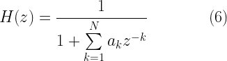
The power law in the power spectrum characterizes the fluctuating observables in many natural systems. Many natural systems exhibit some noise which is a stochastic process with a power spectral density having a power exponent that can take values . Simply put, noise is a colored noise with a power spectral density of over its entire frequency range.
The noise can be classified into different types based on the value of .
Violet noise – = -2, the power spectral density is proportional to . Blue noise – = -1, the power spectral density is proportional to . White noise – = 0, the power spectral density is flat across the whole spectrum. Pink noise – = 1, the power spectral density is proportional to , i.e, it decreases by per octave with increase in frequency. Brownian noise – = 2, the power spectral density is proportional to , therefore it decreases by per octave with increase in frequency.
The power law noise can be generated by sequencing a zero-mean white noise through an auto-regressive (AR) filter of order :
where, is a zero-mean white noise process. Referring the AR generation method described in [3], the coefficients of the AR filter can be generated as
which can be implemented as an infinite impulse response (IIR) filter using the filter transfer function described in equation (6).
The following script implements this method and the sample results are plotted in the next Figure.
The aim of this article is to demonstrate the application of spectral factorization method in generating colored noise having Jakes power spectral density. Before continuing, I urge the reader to go through this post: Introduction to generating correlated Gaussian sequences.
In spectral factorization method, a filter is designed using the desired frequency domain characteristics (like PSD) to transform an uncorrelated Gaussian sequence into a correlated sequence . In the model shown in Figure 1, the input to the LTI system is a white noise whose amplitude follows Gaussian distribution with zero mean and variance and the power spectral density (PSD) of the white noise is a constant across all frequencies.
The white noise sequence drives the LTI system with frequency response producing the signal of interest . The PSD of the output process is therefore
Figure 1: Relationship among various power spectral densities in a filtering process
If the desired power spectral density of the colored noise sequence is given, assuming , the impulse response of the LTI filter can be found by taking the inverse Fourier transform of the frequency response
Once, the impulse response of the filter is obtained, the colored noise sequence can be produced by driving the filter with a zero-mean white noise sequence of unit variance.
Example: Generating colored noise with Jakes PSD
For example, we wish to generate a Gaussian noise sequence whose power spectral density follows the normalized Jakes power spectral density (see section 11.3.2 in the book) given by
Applying spectral factorization method, the frequency response of the desired filter is
The impulse response of the filter is [1]
where, is the fractional Bessel function of the first kind, is the sampling interval for implementing the digital filter and is a constant. The impulse response of the filter can be normalized by dividing by .
The filter can be implemented as a finite impulse response (FIR) filter structure. However, the FIR implementation requires that the impulse response be truncated to a reasonable length. Such truncation leads to ringing effects due to Gibbs phenomenon. To avoid distortions due to truncation, the filter impulse response is usually windowed using a window function such as Hamming window.
where, the Hamming window is defined as
The function given in the book in section 2.6.1 implements a windowed Jakes filterusing the aforementioned equations. The impulse response and the spectral characteristics of the filter are plotted in Figure 2.
Figure 2: Impulse response & spectrum of windowed Jakes filter ( fmax = 10Hz; Ts = 0:01s; N = 512)
A white noise can be transformed into colored noise sequence with Jakes PSD, by processing the white noise through the implemented filter. The script (given in the book in section 2.6.1) illustrates this concept by transforming a white noise sequence into a colored noise sequence. The simulated noise samples and its PSD are plotted in Figure 3.
Key focus: Colored noise sequence (a.k.a correlated Gaussian sequence), is a non-white random sequence, with non-constant power spectral density across frequencies.
Introduction
Speaking of Gaussian random sequences such as Gaussian noise, we generally think that the power spectral density (PSD) of such Gaussian sequences is flat.We should understand that the PSD of a Gausssian sequence need not be flat. This bring out the difference between white and colored random sequences, as captured in Figure 1.
A white noise sequence is defined as any random sequence whose PSD is constant across all frequencies. Gaussian white noise is a Gaussian random sequence, whose amplitude is gaussian distributed and its PSD is a constant. Viewed in another way, a constant PSD in frequency domain implies that the average auto-correlation function in time-domain is an impulse function (Dirac-delta function). That is, the amplitude of noise at any given time instant is correlated only with itself. Therefore, such sequences are also referred as uncorrelated random sequences. White Gaussian noise processes are completely characterized by its mean and variance.
Figure 1: Power spectral densities of white noise and colored noise
A colored noise sequence is simply a non-white random sequence, whose PSD varies with frequency. For a colored noise, the amplitude of noise at any given time instant is correlated with the amplitude of noise occurring at other instants of time. Hence, colored noise sequences will have an auto-correlation function other than the impulse function. Such sequences are also referred as correlated random sequences. Colored Gaussian noise processes are completely characterized by its mean and the shaped of power spectral density (or the shape of auto-correlation function).
In mobile channel model simulations, it is often required to generate correlated Gaussian random sequences with specified mean and power spectral density (like Jakes PSD or Gaussian PSD given in section 11.3.2 in the book). An uncorrelated Gaussian sequence can be transformed into a correlated sequence through filtering or linear transformation, that preserves the Gaussian distribution property of amplitudes, but alters only the correlation property (equivalently the power spectral density). We shall see two methods to generate colored Gaussian noise for given mean and PSD shape
Let’s say we observe a real world signal that has an arbitrary spectrum . We would like to describe the long sequence of using very few parameters, as in applications like linear predictive coding (LPC). The modeling approach, described here, tries to answer the following two questions:
• Is it possible to model the first order (mean/variance) and second order (correlations, spectrum) statistics of the signal just by shaping a white noise spectrum using a transfer function ? (see Figure 1). • Does this produce the same statistics (spectrum, correlations, mean and variance) for a white noise input ?
If the answer is yes to the above two questions, we can simply set the modeled parameters of the system and excite the system with white noise, to produce the desired real world signal. This reduces the amount to data we wish to transmit in a communication system application. This approach can be used to transform an uncorrelated white Gaussian noise sequence to a colored Gaussian noise sequence with desired spectral properties.
The agenda for the subsequent series of articles is to introduce the idea of autocorrelation, AutoCorrelation Function (ACF), Partial AutoCorrelation Function (PACF) , using ACF and PACF in system identification.
Introduction
Given time series data (stock market data, sunspot numbers over a period of years, signal samples received over a communication channel etc.,), successive values in the time series often correlate with each other. This series correlation is termed persistence or inertia and it leads to increased power in the lower frequencies of the frequency spectrum. Persistence can drastically reduces the degrees of freedom in time series modeling (AR, MA , ARMA models). In the test for statistical significance, presence of persistence complicates the test as it reduces the number of independent observations.
Autocorrelation function
Correlation of a time series with its own past and future values- is called autocorrelation. It is also referred as “lagged or series correlation”. Positive autocorrelation is an indication of a specific form of persistence, the tendency of a system to remain in the same state from one observation to the next (example: continuous runs of 0’s or 1’s). If a time series exhibits correlation, the future values of the samples probabilistic-ally depend on the current & past samples. Thus the existence of autocorrelation can be exploited in prediction as well as modeling time series. Autocorrelation can be accessed using the following tools
● Time series plot ● Lagged scatterplot ● AutoCorrelation Function (ACF)
Generating a sample time series
For the purpose of illustration, let’s begin by generating two time series data using Auto-Regressive AR(1) process. AR(1) process relates the current sample x[n] of the output of an LTI system, its immediate past sample x[n-1] and the white noise term w[n].
A generic AR(1) system is given by
Here and are the model parameters which we will tweak to generate different set of time series data and is a constant which will be set to zero . Thus the model can be equivalently written as
Let’s generate two time series data from the above model.
Model 1: a0=0, a1=1
The “Filter” function in Matlab will be utilized to generate the output process x[n]. The filter function, in its basic form – X=filter(B,A,W), takes three inputs. The vectors B and A denote the numerator and denominator co-efficients (model parameters here) of the transfer function of the LTI system in standard difference equation form, W is the white noise vector to the LTI filter and the output of filter is X.
The transfer function of model 1 is therefore,
Where B=1 and A=[1 -1] and the input W is a white noise – which can be generate using randn function. Therefore, the above model can be implemented with the command x=filter(1,[1 -1,randn(1000,1)) generate 1000 samples of x[n]
A=[1 -1];  %model co-effs
% generating using numerator/denominator form with noise
x1 = filter(1,A,randn(1000,1));
plot(x1,’b’);
Model 2: a0=1, a1=0.5
Transfer function of this model is
Where B=1 and A=[1 -0.5] and the input W is a white noise – which can be generated using randn function. Therefore, the above model can be implemented with the command x=filter(1,[1 -0.5], randn(1000,1)) to generate 1000 samples of x[n]
A=[1 -0.5];  %model co-effs
% generating using numerator/denominator form with noise
x2 = filter(1,A,randn(1000,1));
plot(x2,’r’);
Time-series plot of two models – where one model shows persistence and the other does not
In the plot above, the output from model 1 exhibits persistence or positive correlation – positive deviations from mean tend to be followed by positive deviations for some duration and the negative deviations from mean tend to be followed by negative deviations for sometime. When the positive deviations are followed by negative deviations or vice-versa, it is a characteristic of negative correlation. Positive correlations are strong indications of long runs of several consecutive observations above or below mean. Negative correlations indicate low incidence of such runs. The output of the model 2 always jumps around the mean value and there is no consistent departure from the mean – no persistence (no positive correlation). The interpretation of time series plots for clues on persistence is a subjective matter and is left for trained eyes. However, it can be considered as a preliminary analysis.
Persistence – an indication of non-stationarity:
For time series analysis, it is imperative to work with stationary process. Many of the formulated theorems in statistical signal processing assume a series to be stationary (atleast in weak sense). Processes whose Probability Density Functions do not change with time are termed stationary (sub classifications include strict sense stationarity (SSS), weak sense stationarity (WSS) etc.,). For analysis, the joint probability distribution must remain unchanged should there be any shift in the time series. Time series with persistence – changing mean with time – are non-stationary – therefore many theorems in signal processing will not apply as such.
Plotting the histogram of the two series (see next figure) , we can immediately identify that the data generated by model 1 is non-stationary – histogram varies between selected portion of the signal. Whereas, the histogram of the output from model 2 is pretty much same – therefore, this is a stationary signal and is suitable for further analysis.
Persistence – non-stationary and stationary signal
Lagged Scatter Plots
Autocorrelation trend can also be ascertained by lagged scatter plots. In lagged scatter plots, the samples of time series are plotted against one another with one lag at a time. A Strong positive autocorrelation will show of as a linear positive slope for the particular lag value. If the scatter plot is random, it indicates no-correlation for the particular lag.
The scatter plot of the model 1 for the first four lags indicate strong positive correlation at all the four lag values. The scatter plot of model 2 indicates a slightly positive correlation for lag=1 and no correlation for remaining lags. This trend can be clearing seen if we plot the Auto Correlation Function (ACF).
Auto Correlation Function (ACF) or Correlogram
ACF plot summarizes the correlation of a time series at various lags. It plots the correlation co-efficient of the series lagged by 1 delay at a time in the sample plot. Plotting the ACF for the output from both the models with the code below.
[x1c,lags] = xcorr(x1,100,'coeff');
%Plotting only positive lag values - autocorrelation is symmetric
stem(lags(101:end),x1c(101:end));
[x2c,lags] = xcorr(x2,100,'coeff');
stem(lags(101:end),x2c(101:end))
The ACF plot of model 1 indicates strong persistence across all the lags. The ACF plot of model 2 indicates significant correlation only at lag 1 (and lag 0 will obviously correlate fully) which concurs with the lagged scatter plots.
Auto Correlation Function or correlogram
Correlogram has very few significant spikes at very small lags and cuts off drastically/dies down quickly for stationary series. Thus model 2 produces stationary series, where as model 1 does not. Also, model 2 is suitable for further time series analysis.
If a time series data is assumed to be following an Auto-Regressive (AR(N)) model of given form,
the natural tendency is to estimate the model parameters a1,a2,…,aN.
Least squares method can be applied here to estimate the model parameters but the computations become cumbersome as the order N increases.
Fortunately, the AR model co-efficients can be solved for using Yule Walker Equations.
Yule-Walker Equations
Yule Walker equations relate auto-regressive model parameters to auto-covariance rxx[k] of random process x[n]. It can be applied to find the AR(N) model parameters from a given time-series data x[n] that indeed can be assumed to be AR process (visually examining auto-correlation function (ACF) and partial auto-correlation function (PACF) may give clue on whether the data can be assumed as an AR or MA process with appropriate model order N).
Steps to find model parameters using Yule-Walker Equations:
Given x[n], estimate auto-covariance of the process rxx[k]
Solve Yule Walker Equations to find ak(k=0,1,…,N) and σ2 from
To solve Yule-Walker equations, one has to know the model order. Although the Yule-Walker equations can be used to find the model parameters, it cannot give any insight into the model order N directly. Several methods exists to ascertain the model order.
ACF and PACF Autocorrelation Function (ACF) and Partial Autocorrelation Function (PACF) may give insight into the model order of the underlying process
Akaike Information Criterion (AIC)[1] It associates the number of model parameters and the goodness of fit. It also associates a penalty factor to avoid over-fitting (increasing model order always improves the fit – the fitting process has to be stopped somewhere)
Bayesian Information Criterion (BIC)[2] Very similar to AIC
Cross Validation[3] The given time series is broken into subsets. One subset of data is taken at a time and model parameters estimated. The estimated model parameters are cross validated with data from the remaining subsets.
Deriving Yule-Walker Equations
A generic AR model
can be written in compact form as
Note that the scaling factor x[n] term is a0=1
Multiplying (2) by x[n-l]
One can readily identify the auto-correlation and cross-correlation terms as
The next step is to compute the identified cross-correlation rwx[l] term and relate it to the auto-correlation term rxx[l-k]
The term x[n-l] can also be obtained from equation (1) as
Note that data and noise are always uncorrelated, therefore: x[n-k-l]w[n]=0. Also the auto-correlation of noise is zero at all lags except at lag 0 where its value is equal to σ2 (remember the flat Power Spectral Density of white noise and its auto-correlation). These two properties are used in the following steps. Restricting the lags only to positive values and zero ,
Substituting (6) in (4),
Here there are two cases to be solved – l>0 and l=0 For l>0 case, equation (7) becomes,
Clue: notice the lower limit of the summation which changed from k=0 to k=1 .
Now, equation (8) can be written in matrix form
This is the Yule-Walker Equations which comprises of a set of N linear equations and N unknown parameters.
Representing equation (9) in a compact form
The solutions can be solved by
Once we solve for , equivalently ak, – the model parameters, the noise variance σ2 can be found by applying the estimated values of ak in equation (7) by setting l=0
Matlab’s “aryule” efficiently solves the “Yule-Walker” equations using “Levinson Algorithm”[4][5]
Simulation:
Let’s generate an AR(3) process and pretend that we do not anything about the model parameters. We will take this as input data to Yule-Walker and check if it can estimate the model parameters properly
Generating the data from the AR(3) process given above
a=[1  0.9   0.6 0.5]; %model parameters
x=filter(1,a,randn(1000,1)); %data generation with gaussian noise - 1000 samples
plot(x);
title('Sample data from AR(3) process');
xlabel('Sample index');
ylabel('Value');
Figure 1: Simulated data from AR(3) process
Plot the periodogram (PSD plot) for reference. The PSD plots from the estimated model will be checked against this reference plot later.
figure(2);
periodogram(x); hold on; %plot the original frequency response of the data
Running the simulation for three model orders and checking which model order suits the best.
N=[2,3,4];

for i=1:3,
    [a,p] = aryule(x,N(i))
    [H,w]=freqz(sqrt(p),a);
    hp = plot(w/pi,20*log10(2*abs(H)/(2*pi))); %plotting in log scale
end
xlabel('Normalized frequency (\times \pi rad/sample)');
ylabel('One-sided PSD (dB/rad/sample)');
legend('PSD estimate of x','PSD of model output N=2','PSD of model output N=3','PSD of model output N=4');
Figure 2: Power Spectral density of modeled data
The estimated model parameters and the noise variances computed by the Yule-Walker system are given below. It can be ascertained that the estimated parameters are approximately same as that of what is expected. See how the error decreases as the model order N increases. The optimum model order in this case is N=3 since the error has not changed significantly when increasing the order and also the model parameter a4 of the AR(4) process is not-significantly different from zero.
Figure 3: Estimated model parameters and prediction errors for the given model model order
Rate this article: Note: There is a rating embedded within this post, please visit this post to rate it.
Key focus: Can a unique solution exists when solving ARMA (Auto Regressive Moving Average) model ? Apply minimization of squared error to find out.
As discussed in the previous post, the ARMA model is a generalized model that is a mix of both AR and MA model. Given a signal x[n], AR model is easiest to find when compared to finding a suitable ARMA process model. Let’s see why this is so.
AR model error and minimization
In the AR model, the present output sample x[n] and the past N-1 output samples determine the source input w[n]. The difference equation that characterizes this model is given by
The model can be viewed from another perspective, where the input noise w[n] is viewed as an error – the difference between present output sample x[n] and the predicted sample of x[n] from the previous N-1 output samples. Let’s term this “AR model error“. Rearranging the difference equation,
The summation term inside the brackets are viewed as output sample predicted from past N-1 output samples and their difference being the error w[n].
Least squared estimate of the co-efficients – ak are found by evaluating the first derivative of the squared error with respect to ak and equating it to zero – finding the minima.From the equation above, w2[n] is the squared error that we wish to minimize. Here, w2[n] is a quadratic equation of unknown model parameters ak. Quadratic functions have unique minima, therefore it is easier to find the Least Squared Estimates of ak by minimizing w2[n].
ARMA model error and minimization
The difference equation that characterizes this model is given by
Re-arranging, the ARMA model error w[n] is given by
Now, the predictor (terms inside the brackets) considers weighted combinations of past values of both input and output samples.
The squared error, w2[n] is NOT a quadratic function and we have two sets of unknowns – ak and bk. Therefore, no unique solution may be available to minimize this squared error-since multiple minima pose a difficult numerical optimization problem.
Rate this article: Note: There is a rating embedded within this post, please visit this post to rate it.
Key focus: AR, MA & ARMA models express the nature of transfer function of LTI system. Understand the basic idea behind those models & know their frequency responses.
Introduction
Signal models are used to analyze stationary univariate time series. The goal of signal modeling is to estimate the process from which the desired signal is generated. Though the concept described here is related to the topic of “system identification”, they are quite different.
A signal model is an unique combination of a filter and a source input, that may fall into any of the following categories
Filter: state-space model, AR, MA, ARMA (see below)
Source:pulse, pulse train, white noise,…
Motivation
Let’s say we observe a real world signal x[n] that has a spectrum x[ɷ] (the spectrum can be arbitrary – bandpass, baseband etc..,). We would like to describe the long sequence of x[n] using very few parameters (application : Linear Predictive Coding (LPC) ). The modelling approach, described here, tries to answer the following two questions.
Is it possible to model the first order (mean/variance) and second order (correlations, spectrum) statistics of the signal just by shaping a white noise spectrum using a transfer function ? (see Figure 1)
Does this produce the same statistics (spectrum, correlations, mean and variance) for a white noise input ?
If the answer is “yes” to the above two questions, we can simply set the modeled parameters of the system and excite the system with white (flat) noise to produce the desired real world signal. This reduces the amount to data we wish to transmit in a communication system application.
Figure 1: Shaping a white noise spectrum (flat spectrum) to achieve desired spectrum
LTI system model
In the model given below, the random signal x[n] is observed. Given the observed signal x[n], the goal here is to find a model that best describes the spectral properties of x[n] under the following assumptions
● x[n] is WSS (Wide Sense Stationary) and ergodic. ● The input signal to the LTI system is white noise following Gaussian distribution – zero mean and variance σ2. ● The LTI system is BIBO (Bounded Input Bounded Output) stable.
Figure 2: Linear Time Invariant (LTI) system – signal model
In the model shown above, the input to the LTI system is a white noise following Gaussian distribution – zero mean and variance σ2. The power spectral density (PSD) of the noise w[n] is
The noise process drives the LTI system with frequency response H(ejɷ) producing the signal of interest x[n]. The PSD of the output process is therefore,
Three cases are possible given the nature of the transfer function of the LTI system that is under investigation here.
Moving Average (MA) models : H(ejɷ) is an all-zeros system
Auto Regressive Moving Average (ARMA) models : H(ejɷ) is a pole-zero system
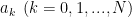
Auto Regressive (AR) models (all-poles model)
In the AR model, the present output sample x[n] and the past N output samples determine the source input w[n]. The difference equation that characterizes this model is given by
Here, the LTI system is an Infinite Impulse Response (IIR) filter. This is evident from the fact that the above equation considered past samples of x[n] when determining w[n], there by creating a feedback loop from the output of the filter.
The frequency response of the IIR filter is well known
Figure 3: Spectrum of all-pole transfer function (representing AR model)
The transfer function H(ejɷ) is an all-pole transfer function (when the denominator is set to zero, the transfer function goes to infinity -> creating peaks in the spectrum). Poles are best suited to model resonant peaks in a given spectrum. At the peaks, the poles are closer to unit circle. This model is well suited for modeling peaky spectra.
In the MA model, the present output sample x[n] is determined by the present source input w[n] and past N samples of source input w[n]. The difference equation that characterizes this model is given by
Here, the LTI system is an Finite Impulse Response (FIR) filter. This is evident from the fact that the above equation that no feedback is involved from output to input.
The frequency response of the FIR filter is well known
The transfer function H(ejɷ) is an all-zero transfer function (when the numerator is set to zero, the transfer function goes to zero -> creating nulls in the spectrum). Zeros are best suited to model sharp nulls in a given spectrum.
Figure 4: Spectrum of all-zeros transfer function (representing MA model)
Auto Regressive Moving Average (ARMA) model (pole-zero model)
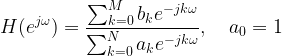
ARMA model is a generalized model that is a combination of AR and MA model. The output of the filter is linear combination of both weighted inputs (present and past samples) and weight outputs (present and past samples). The difference equation that characterizes this model is given by
The frequency response of this generalized filter is well known
The transfer function H(ejɷ) is a pole-zero transfer function. It is best suited for modelling complex spectra having well defined resonant peaks and nulls.
This website uses cookies to improve your experience while you navigate through the website. Out of these, the cookies that are categorized as necessary are stored on your browser as they are essential for the working of basic functionalities of the website. We also use third-party cookies that help us analyze and understand how you use this website. These cookies will be stored in your browser only with your consent. You also have the option to opt-out of these cookies. But opting out of some of these cookies may affect your browsing experience.
Necessary cookies are absolutely essential for the website to function properly. These cookies ensure basic functionalities and security features of the website, anonymously.
Cookie
Duration
Description
cookielawinfo-checbox-analytics
11 months
This cookie is set by GDPR Cookie Consent plugin. The cookie is used to store the user consent for the cookies in the category "Analytics".
cookielawinfo-checbox-analytics
11 months
This cookie is set by GDPR Cookie Consent plugin. The cookie is used to store the user consent for the cookies in the category "Analytics".
cookielawinfo-checbox-functional
11 months
The cookie is set by GDPR cookie consent to record the user consent for the cookies in the category "Functional".
cookielawinfo-checbox-functional
11 months
The cookie is set by GDPR cookie consent to record the user consent for the cookies in the category "Functional".
cookielawinfo-checbox-others
11 months
This cookie is set by GDPR Cookie Consent plugin. The cookie is used to store the user consent for the cookies in the category "Other.
cookielawinfo-checbox-others
11 months
This cookie is set by GDPR Cookie Consent plugin. The cookie is used to store the user consent for the cookies in the category "Other.
cookielawinfo-checkbox-necessary
11 months
This cookie is set by GDPR Cookie Consent plugin. The cookies is used to store the user consent for the cookies in the category "Necessary".
cookielawinfo-checkbox-performance
11 months
This cookie is set by GDPR Cookie Consent plugin. The cookie is used to store the user consent for the cookies in the category "Performance".
viewed_cookie_policy
11 months
The cookie is set by the GDPR Cookie Consent plugin and is used to store whether or not user has consented to the use of cookies. It does not store any personal data.
Functional cookies help to perform certain functionalities like sharing the content of the website on social media platforms, collect feedbacks, and other third-party features.
Performance cookies are used to understand and analyze the key performance indexes of the website which helps in delivering a better user experience for the visitors.
Analytical cookies are used to understand how visitors interact with the website. These cookies help provide information on metrics the number of visitors, bounce rate, traffic source, etc.

![x[n]](https://s0.wp.com/latex.php?latex=x%5Bn%5D&bg=ffffff&fg=000&s=0&c=20201002)

![y[n]](https://s0.wp.com/latex.php?latex=y%5Bn%5D&bg=ffffff&fg=000&s=0&c=20201002)


![R_{yy}[k]](https://s0.wp.com/latex.php?latex=R_%7Byy%7D%5Bk%5D&bg=ffffff&fg=000&s=0&c=20201002)

![R_{yy}[n]](https://s0.wp.com/latex.php?latex=R_%7Byy%7D%5Bn%5D&bg=ffffff&fg=000&s=0&c=20201002)


![\sum_{k=0}^{k=N} a_k y[n - k] = x[n] \quad \quad \quad \quad (8)](https://s0.wp.com/latex.php?latex=%5Csum_%7Bk%3D0%7D%5E%7Bk%3DN%7D+a_k+y%5Bn+-+k%5D+%3D+x%5Bn%5D+%5Cquad+%5Cquad+%5Cquad+%5Cquad+%288%29+&bg=ffffff&fg=000&s=2&c=20201002)


![h[n]](https://s0.wp.com/latex.php?latex=h%5Bn%5D&bg=ffffff&fg=000&s=0&c=20201002)


![H(f) = \sqrt{S_{yy}(f)} = \sqrt{\pi f_{max}} \left[1- \left(f/f_{max}\right)^2\right]^{-1/4} \quad (5)](https://s0.wp.com/latex.php?latex=H%28f%29+%3D+%5Csqrt%7BS_%7Byy%7D%28f%29%7D+%3D+%5Csqrt%7B%5Cpi+f_%7Bmax%7D%7D+%5Cleft%5B1-+%5Cleft%28f%2Ff_%7Bmax%7D%5Cright%29%5E2%5Cright%5D%5E%7B-1%2F4%7D+%5Cquad+%285%29+&bg=ffffff&fg=000&s=2&c=20201002)

![h[n] = C f_{max} x^{-1/4} J_{1/4} (x) , \quad \quad x = 2 \pi f_{max} |n T_s| \quad (6)](https://s0.wp.com/latex.php?latex=h%5Bn%5D+%3D+C+f_%7Bmax%7D+x%5E%7B-1%2F4%7D+J_%7B1%2F4%7D+%28x%29+%2C+%5Cquad+%5Cquad+x+%3D+2+%5Cpi+f_%7Bmax%7D+%7Cn+T_s%7C+%5Cquad+%286%29+&bg=ffffff&fg=000&s=2&c=20201002)


![h_{norm}[n] = x^{-1/4} J_{1/4} (x), \quad \quad x = 2 \pi f_{max} |n T_s| \quad (7)](https://s0.wp.com/latex.php?latex=h_%7Bnorm%7D%5Bn%5D+%3D+x%5E%7B-1%2F4%7D+J_%7B1%2F4%7D+%28x%29%2C+%5Cquad+%5Cquad+x+%3D+2+%5Cpi+f_%7Bmax%7D+%7Cn+T_s%7C+%5Cquad+%287%29+&bg=ffffff&fg=000&s=2&c=20201002)

![h_{w}[n] = h_{norm}[n] w_{H}[n] \quad \quad (8)](https://s0.wp.com/latex.php?latex=h_%7Bw%7D%5Bn%5D+%3D+h_%7Bnorm%7D%5Bn%5D+w_%7BH%7D%5Bn%5D+%5Cquad+%5Cquad+%288%29+&bg=ffffff&fg=000&s=2&c=20201002)

![w_{H}[n] = 0.54-0.46 \; cos(2 \pi n /N) \quad \quad (9)](https://s0.wp.com/latex.php?latex=w_%7BH%7D%5Bn%5D+%3D+0.54-0.46+%5C%3B+cos%282+%5Cpi+n+%2FN%29+%5Cquad+%5Cquad+%289%29+&bg=ffffff&fg=000&s=2&c=20201002)


![a_0x[n]= c + a_1 x[n-1] + w[n] \quad\quad ,w[n] \sim N(0,\sigma^2)](https://s0.wp.com/latex.php?latex=a_0x%5Bn%5D%3D+c%C2%A0%2B+a_1+x%5Bn-1%5D+%2B+w%5Bn%5D+%C2%A0%5Cquad%5Cquad+%2Cw%5Bn%5D+%5Csim+N%280%2C%5Csigma%5E2%29+&bg=ffffff&fg=000&s=2&c=20201002)


![a_0x[n]- a_1 x[n-1] = w[n] \quad\quad ,w[n] \sim N(0,\sigma^2)](https://s0.wp.com/latex.php?latex=a_0x%5Bn%5D-+a_1+x%5Bn-1%5D+%C2%A0%3D+w%5Bn%5D+%C2%A0%5Cquad%5Cquad+%2Cw%5Bn%5D+%5Csim+N%280%2C%5Csigma%5E2%29+&bg=ffffff&fg=000&s=2&c=20201002)

![x[n]- x[n-1] = w[n] \quad\quad ,w[n] \sim N(0,\sigma^2)](https://s0.wp.com/latex.php?latex=x%5Bn%5D-+x%5Bn-1%5D+%3D+w%5Bn%5D+%C2%A0%5Cquad%5Cquad+%2Cw%5Bn%5D+%5Csim+N%280%2C%5Csigma%5E2%29+&bg=ffffff&fg=000&s=2&c=20201002)


![x[n]- 0.5 x[n-1] = w[n] \quad\quad w[n] \sim N(0,\sigma^2)](https://s0.wp.com/latex.php?latex=x%5Bn%5D-+0.5+x%5Bn-1%5D+%3D+w%5Bn%5D+%C2%A0%5Cquad%5Cquad+w%5Bn%5D+%5Csim+N%280%2C%5Csigma%5E2%29+&bg=ffffff&fg=000&s=2&c=20201002)


![x[n] + a_1 x[n-1] + a_2 x[n-2] + \cdots + a_N x[n-N] = w[n]](https://s0.wp.com/latex.php?latex=x%5Bn%5D+%2B+a_1+x%5Bn-1%5D+%2B+a_2+x%5Bn-2%5D+%2B+%5Ccdots+%2B+a_N+x%5Bn-N%5D+%3D+w%5Bn%5D+&bg=ffffff&fg=000&s=1&c=20201002)

![\hat{r}_{xx}[k]](https://s0.wp.com/latex.php?latex=%5Chat%7Br%7D_%7Bxx%7D%5Bk%5D&bg=ffffff&fg=000&s=0&c=20201002)

![x[n] + a_1 x[n-1] + a_2 x[n-2] + \cdots + a_N x[n-N] = w[n] \quad\quad (1)](https://s0.wp.com/latex.php?latex=x%5Bn%5D+%2B+a_1+x%5Bn-1%5D+%2B+a_2+x%5Bn-2%5D+%2B+%5Ccdots+%2B+a_N+x%5Bn-N%5D+%3D+w%5Bn%5D+%5Cquad%5Cquad+%281%29+&bg=ffffff&fg=000&s=1&c=20201002)

![\displaystyle{\sum_{k=0}^{N} a_k x[n-k]=w[n], \;\;\; a_0=1} \quad\quad (2)](https://s0.wp.com/latex.php?latex=%5Cdisplaystyle%7B%5Csum_%7Bk%3D0%7D%5E%7BN%7D+a_k+x%5Bn-k%5D%3Dw%5Bn%5D%2C+%5C%3B%5C%3B%5C%3B+a_0%3D1%7D+%5Cquad%5Cquad+%282%29+&bg=ffffff&fg=000&s=1&c=20201002)

![\displaystyle{ \sum_{k=0}^{N} a_k E\left\{ x[n-k]x[n-l] \right\}=E \left\{ w[n]x[n-l] \right\}, \;\;\; a_0=1} \quad\quad (3)](https://s0.wp.com/latex.php?latex=%5Cdisplaystyle%7B+%5Csum_%7Bk%3D0%7D%5E%7BN%7D+a_k+E%5Cleft%5C%7B+x%5Bn-k%5Dx%5Bn-l%5D+%5Cright%5C%7D%3DE+%5Cleft%5C%7B+w%5Bn%5Dx%5Bn-l%5D+%5Cright%5C%7D%2C+%5C%3B%5C%3B%5C%3B+a_0%3D1%7D+%5Cquad%5Cquad++%283%29&bg=ffffff&fg=000&s=1&c=20201002)


![\displaystyle{\sum_{k=0}^{N} a_k \underbrace{E\left\{ x[n-k] x[n-l]\right\}}_{r_{xx}(l-k)} = \underbrace{E\left\{ w[n] x[n-l]\right\}}_{r_{wx}(l)}}](https://s0.wp.com/latex.php?latex=%5Cdisplaystyle%7B%5Csum_%7Bk%3D0%7D%5E%7BN%7D+a_k+%5Cunderbrace%7BE%5Cleft%5C%7B+x%5Bn-k%5D+x%5Bn-l%5D%5Cright%5C%7D%7D_%7Br_%7Bxx%7D%28l-k%29%7D+%3D+%5Cunderbrace%7BE%5Cleft%5C%7B+w%5Bn%5D+x%5Bn-l%5D%5Cright%5C%7D%7D_%7Br_%7Bwx%7D%28l%29%7D%7D+&bg=ffffff&fg=000&s=1&c=20201002)

![\displaystyle{\sum_{k=0}^{N} a_k r_{xx}[l-k]=r_{wx}[l]}, \;\;\; a_0=1 \quad\quad (4)](https://s0.wp.com/latex.php?latex=%5Cdisplaystyle%7B%5Csum_%7Bk%3D0%7D%5E%7BN%7D+a_k+r_%7Bxx%7D%5Bl-k%5D%3Dr_%7Bwx%7D%5Bl%5D%7D%2C+%5C%3B%5C%3B%5C%3B+a_0%3D1+%5Cquad%5Cquad+%284%29+&bg=ffffff&fg=000&s=1&c=20201002)

![\displaystyle{x[n-l]=-\sum_{k=1}^{N} a_k x[n-k-l]+w[n-l]} \quad\quad (5)](https://s0.wp.com/latex.php?latex=%5Cdisplaystyle%7Bx%5Bn-l%5D%3D-%5Csum_%7Bk%3D1%7D%5E%7BN%7D+a_k+x%5Bn-k-l%5D%2Bw%5Bn-l%5D%7D+%5Cquad%5Cquad+%285%29+&bg=ffffff&fg=000&s=1&c=20201002)

![\displaystyle{ \begin{aligned} r_{wx}(l) &=E \left\{ w[n]x[n-l] \right\} \\ &= E \left\{ w[n] \left ( -\sum_{k=1}^{N} a_kx[n-k-l]+w[n-l] \right ) \right\}\\ &= E\left \{ -\sum_{k=1}^{N} a_kx[n-k-l]w[n]+w[n-l]w[n] \right \} \\ &= E\left \{ 0 + w[n-l]w[n] \right \}\\ &= E\left \{ w[n-l]w[n] \right \}\\ &=\begin{cases}0 \;\; ,l>0 \\ \sigma^2 \;,l=0\end{cases} \end{aligned}} \quad\quad (6)](https://s0.wp.com/latex.php?latex=%5Cdisplaystyle%7B+%5Cbegin%7Baligned%7D+r_%7Bwx%7D%28l%29+%26%3DE+%5Cleft%5C%7B+w%5Bn%5Dx%5Bn-l%5D+%5Cright%5C%7D+%5C%5C+%26%3D+E+%5Cleft%5C%7B+w%5Bn%5D+%5Cleft+%28+-%5Csum_%7Bk%3D1%7D%5E%7BN%7D+a_kx%5Bn-k-l%5D%2Bw%5Bn-l%5D+%5Cright+%29+%5Cright%5C%7D%5C%5C+%26%3D+E%5Cleft+%5C%7B+-%5Csum_%7Bk%3D1%7D%5E%7BN%7D+a_kx%5Bn-k-l%5Dw%5Bn%5D%2Bw%5Bn-l%5Dw%5Bn%5D+%5Cright+%5C%7D+%5C%5C+%26%3D+E%5Cleft+%5C%7B+0+%2B+w%5Bn-l%5Dw%5Bn%5D+%5Cright+%5C%7D%5C%5C+%26%3D+E%5Cleft+%5C%7B+w%5Bn-l%5Dw%5Bn%5D+%5Cright+%5C%7D%5C%5C+%26%3D%5Cbegin%7Bcases%7D0+%5C%3B%5C%3B+%2Cl%3E0+%5C%5C+%5Csigma%5E2+%5C%3B%2Cl%3D0%5Cend%7Bcases%7D+%5Cend%7Baligned%7D%7D+%5Cquad%5Cquad+%286%29+&bg=ffffff&fg=000&s=1&c=20201002)

![\displaystyle{\sum_{k=0}^{N} a_kr_{xx}[l-k]=\begin{cases}0 \;\; ,l>0 \\ \sigma^2 \;,l=0\end{cases} },\;\;\; a_0=1 \quad\quad (7)](https://s0.wp.com/latex.php?latex=%5Cdisplaystyle%7B%5Csum_%7Bk%3D0%7D%5E%7BN%7D+a_kr_%7Bxx%7D%5Bl-k%5D%3D%5Cbegin%7Bcases%7D0+%5C%3B%5C%3B+%2Cl%3E0+%5C%5C+%5Csigma%5E2+%5C%3B%2Cl%3D0%5Cend%7Bcases%7D+%7D%2C%5C%3B%5C%3B%5C%3B+a_0%3D1+%5Cquad%5Cquad+%287%29+&bg=ffffff&fg=000&s=1&c=20201002)

![\displaystyle{ \sum_{k=1}^{N} a_k r_{xx}[l-k]=-r_{xx}[l]} \quad\quad (8)](https://s0.wp.com/latex.php?latex=%5Cdisplaystyle%7B+%5Csum_%7Bk%3D1%7D%5E%7BN%7D+a_k+r_%7Bxx%7D%5Bl-k%5D%3D-r_%7Bxx%7D%5Bl%5D%7D+%5Cquad%5Cquad+%288%29+&bg=ffffff&fg=000&s=1&c=20201002)


![x[n] = -0.9 x[n-1] -0.6 x[n-2] -0.5 x[n-3]](https://s0.wp.com/latex.php?latex=x%5Bn%5D+%3D+-0.9+x%5Bn-1%5D+-0.6+x%5Bn-2%5D+-0.5+x%5Bn-3%5D+&bg=ffffff&fg=000&s=1&c=20201002)


![\displaystyle{ w[n]= x[n]-\left(-\sum^{N}_{k=1}a_k x[n-k] \right)}](https://s0.wp.com/latex.php?latex=%5Cdisplaystyle%7B+w%5Bn%5D%3D+x%5Bn%5D-%5Cleft%28-%5Csum%5E%7BN%7D_%7Bk%3D1%7Da_k+x%5Bn-k%5D+%5Cright%29%7D+&bg=ffffff&fg=000&s=1&c=20201002)


![\begin{aligned} x[n] + a_1 x[n-1] + \cdots + a_N x[n-N] = & b_0 w[n] + b_1 w[n-1] + \\ & \cdots + b_M w[n-M] \end{aligned}](https://s0.wp.com/latex.php?latex=%5Cbegin%7Baligned%7D+x%5Bn%5D+%2B+a_1+x%5Bn-1%5D+%2B+%5Ccdots+%2B+a_N+x%5Bn-N%5D+%3D+%26+b_0+w%5Bn%5D+%2B+b_1+w%5Bn-1%5D+%2B+%5C%5C+%26+%5Ccdots+%2B+b_M+w%5Bn-M%5D+%5Cend%7Baligned%7D&bg=ffffff&fg=000&s=1&c=20201002)

![\displaystyle{ w[n]= x[n]-\left(-\sum^{N}_{k=1}a_k x[n-k] + \sum^{M}_{k=1}b_k w[n-k] \right)}](https://s0.wp.com/latex.php?latex=%5Cdisplaystyle%7B+w%5Bn%5D%3D+x%5Bn%5D-%5Cleft%28-%5Csum%5E%7BN%7D_%7Bk%3D1%7Da_k+x%5Bn-k%5D+%2B+%5Csum%5E%7BM%7D_%7Bk%3D1%7Db_k+w%5Bn-k%5D+%5Cright%29%7D+&bg=ffffff&fg=000&s=1&c=20201002)


![x[n] = b_0 w[n] + b_1 w[n-1] + b_2 w[n-2] + \cdots + b_M w[n-M]](https://s0.wp.com/latex.php?latex=x%5Bn%5D+%3D+b_0+w%5Bn%5D+%2B+b_1+w%5Bn-1%5D+%2B+b_2+w%5Bn-2%5D+%2B+%5Ccdots+%2B+b_M+w%5Bn-M%5D++&bg=ffffff&fg=000&s=1&c=20201002)


![x[n] + a_1 x[n-1] + \cdots + a_N x[n-N] = b_0 w[n] + b_1 w[n-1] + \cdots + b_M w[n-M]](https://s0.wp.com/latex.php?latex=x%5Bn%5D+%2B+a_1+x%5Bn-1%5D+%2B+%5Ccdots+%2B+a_N+x%5Bn-N%5D+%3D+b_0+w%5Bn%5D+%2B+b_1+w%5Bn-1%5D+%2B+%5Ccdots+%2B+b_M+w%5Bn-M%5D+&bg=ffffff&fg=000&s=1&c=20201002)