Simulate additive white Gaussian noise (AWGN) channel

In this article, the relationship between SNR-per-bit (Eb/N0) and SNR-per-symbol (Es/N0) are defined with respect to M-ary signaling schemes. Then the complex baseband model for an AWGN channel is discussed, followed by the theoretical error rates of various modulations over the additive white Gaussian noise (AWGN) channel. Finally, the complex baseband models for digital modulators and detectors developed in previous chapter of this book, are incorporated to build a complete communication system model.

If you would like to know more about the simulation and analysis of white noise, I urge you to read this article: White noise: Simulation & Analysis using Matlab.

Signal to noise ratio (SNR) definitions

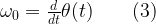
Assuming a channel of bandwidth B, received signal power Pr and the power spectral density (PSD) of noise N0/2, the signal to noise ratio (SNR) is given by

Let a signal’s energy-per-bit is denoted as Eb and the energy-per-symbol as Es, then γb=Eb/N0 and γs=Es/N0 are the SNR-per-bit and the SNR-per-symbol respectively.

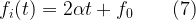
For uncoded M-ary signaling scheme with k = log2(M) bits per symbol, the signal energy per modulated symbol is given by

The SNR per symbol is given by

AWGN channel model

In order to simulate a specific SNR point in performance simulations, the modulated signal from the transmitter needs to be added with random noise of specific strength. The strength of the generated noise depends on the desired SNR level which usually is an input in such simulations. In practice, SNRs are specified in dB. Given a specific SNR point for simulation, let’s see how we can simulate an AWGN channel that adds correct level of white noise to the transmitted symbols.

simulation model for additive white Gaussian noise (awgn) channel
Figure 1: Simplified simulation model for awgn channel

Consider the AWGN channel model given in Figure 1. Given a specific SNR point to simulate, we wish to generate a white Gaussian noise vector of appropriate strength and add it to the incoming signal. The method described can be applied for both waveform simulations and the complex baseband simulations. In following text, the term SNR (γ) refers to γb = Eb/N0 when the modulation is of binary type (example: BPSK). For multilevel modulations such as QPSK and MQAM, the term SNR refers to γs = Es/N0.

(1) Assume, s is a vector that represents the transmitted signal. We wish to generate a vector r that represents the signal after passing through the AWGN channel. The amount of noise added by the AWGN channel is controlled by the given SNR – γ

(2) For waveform simulation model, let the given oversampling ratio is denoted as L. On the other hand, if you are using the complex baseband models, set L=1.

(3) Let N denotes the length of the vector s. The signal power for the vector s can be measured as,

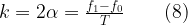
(4) The required power spectral density of the noise vector n is computed as

(5) Assuming complex IQ plane for all the digital modulations, the required noise variance (noise power) for generating Gaussian random noise is given by

(6) Generate the noise vector n drawn from normal distribution with mean set to zero and the standard deviation computed from the equation given above

(7) Finally add the generated noise vector (n) to the signal (s)

Matlab code

The following custom function written in Matlab, can be used for adding AWGN noise to an incoming signal. It can be used in waveform simulation as well as complex baseband simulation models.

%author - Mathuranathan Viswanathan (gaussianwaves.com
%This code is part of the books: Wireless communication systems using Matlab & Digital modulations using Matlab.

function [r,n,N0] = add_awgn_noise(s,SNRdB,L)
%Function to add AWGN to the given signal
%[r,n,N0]= add_awgn_noise(s,SNRdB) adds AWGN noise vector to signal
%'s' to generate a %resulting signal vector 'r' of specified SNR
%in dB. It also returns the noise vector 'n' that is added to the
%signal 's' and the spectral density N0 of noise added
%
%[r,n,N0]= add_awgn_noise(s,SNRdB,L) adds AWGN noise vector to
%signal 's' to generate a resulting signal vector 'r' of specified
%SNR in dB. The parameter 'L' specifies the oversampling ratio used
%in the system (for waveform simulation). It also returns the noise
%vector 'n' that is added to the signal 's' and the spectral
%density N0 of noise added
 s_temp=s;
 if iscolumn(s), s=s.'; end; %to return the result in same dim as 's'
 gamma = 10ˆ(SNRdB/10); %SNR to linear scale
 
 if nargin==2, L=1; end %if third argument is not given, set it to 1
 
 if isvector(s),
  P=L*sum(abs(s).ˆ2)/length(s);%Actual power in the vector
 else %for multi-dimensional signals like MFSK
  P=L*sum(sum(abs(s).ˆ2))/length(s); %if s is a matrix [MxN]
 end
 
 N0=P/gamma; %Find the noise spectral density
 if(isreal(s)),
  n = sqrt(N0/2)*randn(size(s));%computed noise
 else
  n = sqrt(N0/2)*(randn(size(s))+1i*randn(size(s)));%computed noise
 end
 
 r = s + n; %received signal
 
 if iscolumn(s_temp), r=r.'; end;%return r in original format as s
end

Python code

The following custom function written in Python 3, can be used for adding AWGN noise to an incoming signal. It can be used in waveform simulation as well as complex baseband simulation models.

# author - Mathuranathan Viswanathan (gaussianwaves.com
# This code is part of the book Digital Modulations using Python

from numpy import sum,isrealobj,sqrt
from numpy.random import standard_normal

def awgn(s,SNRdB,L=1):
    """
    AWGN channel
    Add AWGN noise to input signal. The function adds AWGN noise vector to signal 's' to generate a resulting signal vector 'r' of specified SNR in dB. It also
    returns the noise vector 'n' that is added to the signal 's' and the power spectral density N0 of noise added
    Parameters:
        s : input/transmitted signal vector
        SNRdB : desired signal to noise ratio (expressed in dB) for the received signal
        L : oversampling factor (applicable for waveform simulation) default L = 1.
    Returns:
        r : received signal vector (r=s+n)
"""
    gamma = 10**(SNRdB/10) #SNR to linear scale
    if s.ndim==1:# if s is single dimensional vector
        P=L*sum(abs(s)**2)/len(s) #Actual power in the vector
    else: # multi-dimensional signals like MFSK
        P=L*sum(sum(abs(s)**2))/len(s) # if s is a matrix [MxN]
    N0=P/gamma # Find the noise spectral density
    if isrealobj(s):# check if input is real/complex object type
        n = sqrt(N0/2)*standard_normal(s.shape) # computed noise
    else:
        n = sqrt(N0/2)*(standard_normal(s.shape)+1j*standard_normal(s.shape))
    r = s + n # received signal
return r

Theoretical symbol error rates for digital modulations in AWGN channel

Denoting the symbol error rate (SER) as , SNR-per-bit as and SNR-per-symbol as , the symbol error rates for various modulation schemes over AWGN channel are listed in Table 1 (refer [1]).

Table 1: Theoretical symbol error rate for various modulations in AWGN channel

The theoretical symbol error rates are coded as a reusable function. In this implementation, erfc function is used instead of the Q function shown in the Table 4.1. The following equation describes the relationship between the erfc function and the Q function.

Unified simulation model for performance simulation

In the previous chapter of the books, the code implementation for complex baseband models for various digital modulators and demodulator are given. Using these models, we can create a unified simulation code for simulating the performance of various modulation techniques over AWGN channel.

The complete simulation model for performance simulation over AWGN channel is given in Figure 2. The figure is illustrated for a coherent communication system model (applicable for MPSK/MQAM/MPAM modulations)

Figure 2: Complete simulation model for a communication system with AWGN channel

The Matlab code implementing the aforementioned simulation model is given in the books. Here, an unified approach is employed to simulate the performance of any of the given modulation technique – MPSK, MQAM, MPAM or MFSK (MFSK simulation technique is available in the following books: Digital Modulations using Python and Digital Modulations using Matlab).

This article is part of the following books
Digital Modulations using Matlab : Build Simulation Models from Scratch, ISBN: 978-1521493885
Digital Modulations using Python ISBN: 978-1712321638
Wireless communication systems in Matlab ISBN: 979-8648350779
All books available in ebook (PDF) and Paperback formats

The simulation code will automatically choose the selected modulation type, performs Monte Carlo simulation, computes symbol error rates and plots them against the theoretical symbol error rates. The simulated performance results obtained for MQAM and MPSK modulations are shown in the Figure 3 and Figure 4.

Figure 3: Simulated symbol error rate performance of M-QAM modulation over AWGN channel

Rate this article: Note: There is a rating embedded within this post, please visit this post to rate it.

References

[1] Andrea Goldsmith, Wireless Communications, Cambridge University Pres, first edition, August 8, 2005.↗

Books by the author


Wireless Communication Systems in Matlab
Second Edition(PDF)

Note: There is a rating embedded within this post, please visit this post to rate it.
Checkout Added to cart

Digital Modulations using Python
(PDF ebook)

Note: There is a rating embedded within this post, please visit this post to rate it.
Checkout Added to cart

Digital Modulations using Matlab
(PDF ebook)

Note: There is a rating embedded within this post, please visit this post to rate it.
Checkout Added to cart
Hand-picked Best books on Communication Engineering
Best books on Signal Processing

Construct autocorrelation Matrix in Matlab & Python

Auto-correlation, also called series correlation, is the correlation of a given sequence with itself as a function of time lag. Cross-correlation is a more generic term, which gives the correlation between two different sequences as a function of time lag.

Given two sequences and , the cross-correlation at times separated by lag i is given by ( denotes complex conjugate operation)

Auto-correlation is a special case of cross-correlation, where x=y. One can use a brute force method (using for loops implementing the above equation) to compute the auto-correlation sequence. However, other alternatives are also at your disposal.

Method 1: Auto-correlation using xcorr function

Matlab

For a N-dimensional given vector x, the Matlab command xcorr(x,x) or simply xcorr(x) gives the auto-correlation sequence. For the input sequence x=[1,2,3,4], the command xcorr(x) gives the following result.

>> x=[1 2 3 4]
>> acf=xcorr(x)
acf= 4   11   20   30   20   11  4

Python

In Python, autocorrelation of 1-D sequence can be obtained using numpy.correlate function. Set the parameter mode=’full’ which is useful for calculating the autocorrelation as a function of lag.

import numpy as np
x = np.asarray([1,2,3,4])
np.correlate(x, x,mode='full')
# output: array([ 4, 11, 20, 30, 20, 11,  4])

Method 2: Auto-correlation using Convolution

Auto-correlation sequence can be computed as the convolution between the given sequence and the reversed (flipped) version of the conjugate of the sequence.The conjugate operation is not needed if the input sequence is real.

Matlab

>> x=[1 2 3 4]
>> acf=conv(x,fliplr(conj(x)))
acf= 4   11   20   30   20   11  4

Python

import numpy as np
x = np.asarray([1,2,3,4])
np.convolve(x,np.conj(x)[::-1])
# output: array([ 4, 11, 20, 30, 20, 11,  4])

Method 3: Autocorrelation using Toeplitz matrix

Autocorrelation sequence can be found using Toeplitz matrices. An example for using Toeplitz matrix structure for computing convolution is given here. The same technique is extended here, where one signal is set as input sequence and the other is just the flipped version of its conjugate. The conjugate operation is not needed if the input sequence is real.

Matlab

>> x=[1 2 3 4]
>> acf=toeplitz([x zeros(1,length(x)-1)],[x(1) zeros(1,length(conj(x))-1)])*fliplr(x).'
acf= 4   11   20   30   20   11  4

Python

import numpy as np
from scipy.linalg import toeplitz
x = np.asarray([1,2,3,4])
toeplitz(np.pad(x, (0,len(x)-1),mode='constant'),np.pad([x[0]], (0,len(x)-1),mode='constant'))@x[::-1]
# output: array([ 4, 11, 20, 30, 20, 11, 4])

Method 4: Auto-correlation using FFT/IFFT

Auto-correlation sequence can be found using FFT/IFFT pairs. An example for using FFT/IFFT for computing convolution is given here. The same technique is extended here, where one signal is set as input sequence and the other is just the flipped version of its conjugate.The conjugate operation is not needed if the input sequence is real.

Matlab

>> x=[1 2 3 4]
>> L = 2*length(x)-1
>> acf=ifft(fft(x,L).*fft(fliplr(conj(x)),L))
acf= 4   11   20   30   20   11  4

Python

import numpy as np
from scipy.fftpack import fft,ifft

x = np.asarray([1,2,3,4])

L = 2*len(x) - 1
ifft(fft(x,L)*fft(np.conj(x)[::-1],L))
#output: array([ 4+0j, 11+0j, 20+0j, 30+0j, 20+0j, 11+0j, 4+0j])

Note that in all the above cases, due to the symmetry property of auto-correlation function, the center element represents .

Construction the Auto-correlation Matrix

Auto-correlation matrix is a special form of matrix constructed from auto-correlation sequence. It takes the following form.

The auto-correlation matrix is easily constructed, once the auto-correlation sequence is known. The auto-correlation matrix is a Hermitian matrix as well as a Toeplitz matrix. This property is exploited in the following code for constructing the Auto-Correlation matrix.

Matlab

>> x=[1+j 2+j 3-j] %x is complex
>> acf=conv(x,fliplr(conj(x)))% %using Method 2 to compute Auto-correlation sequence
>>Rxx=acf(3:end); % R_xx(0) is the center element
>>Rx=toeplitz(Rxx,[Rxx(1) conj(Rxx(2:end))])

Python

import numpy as np
x = np.asarray([1+1j,2+1j,3-1j]) #x is complex
acf = np.convolve(x,np.conj(x)[::-1]) # using Method 2 to compute Auto-correlation sequence
Rxx=acf[2:]; # R_xx(0) is the center element
Rx = toeplitz(Rxx,np.hstack((Rxx[0], np.conj(Rxx[1:]))))

Result:

Rate this article: Note: There is a rating embedded within this post, please visit this post to rate it.

References:

[1] Reddi.S.S,”Eigen Vector properties of Toeplitz matrices and their application to spectral analysis of time series, Signal Processing, Vol 7,North-Holland, 1984,pp 46-56.↗
[2] Robert M. Gray,”Toeplitz and circulant matrices – an overview”,Department of Electrical Engineering,Stanford University,Stanford 94305,USA.↗
[3] Matlab documentation help on Toeplitz command.↗

Books by the author


Wireless Communication Systems in Matlab
Second Edition(PDF)

Note: There is a rating embedded within this post, please visit this post to rate it.
Checkout Added to cart

Digital Modulations using Python
(PDF ebook)

Note: There is a rating embedded within this post, please visit this post to rate it.
Checkout Added to cart

Digital Modulations using Matlab
(PDF ebook)

Note: There is a rating embedded within this post, please visit this post to rate it.
Checkout Added to cart
Hand-picked Best books on Communication Engineering
Best books on Signal Processing

Chirp Signal – FFT & PSD in Matlab & Python

Key focus: Know how to generate a Chirp signal, compute its Fourier Transform using FFT and power spectral density (PSD) in Matlab & Python.

This article is part of the following books
Digital Modulations using Matlab : Build Simulation Models from Scratch, ISBN: 978-1521493885
Digital Modulations using Python ISBN: 978-1712321638
Wireless communication systems in Matlab ISBN: 979-8648350779
All books available in ebook (PDF) and Paperback formats

Introduction

All the signals discussed so far do not change in frequency over time. Obtaining a signal with time-varying frequency is of main focus here. A signal that varies in frequency over time is called “chirp”. The frequency of the chirp signal can vary from low to high frequency (up-chirp) or from high to low frequency (low-chirp).

Observation

Chirp signals/signatures are encountered in many applications ranging from radar, sonar, spread spectrum, optical communication, image processing, doppler effect, motion of a pendulum, as gravitation waves, manifestation as Frequency Modulation (FM), echo location [1] etc.

Mathematical Description:

A linear chirp signal sweeps the frequency from low to high frequency (or vice-versa) linearly. One approach to generate a chirp signal is to concatenate a series of segments of sine waves each with increasing(or decreasing) frequency in order. This method introduces discontinuities in the chirp signal due to the mismatch in the phases of each such segments. Modifying the equation of a sinusoid to generate a chirp signal is a better approach.

The equation for generating a sinusoidal (cosine here) signal with amplitude A, angular frequency and initial phase is

This can be written as a function of instantaneous phase

where is the instantaneous phase of the sinusoid and it is linear in time. The time derivative of instantaneous phase is equal to the angular frequency of the sinusoid – which in case is a constant in the above equation.

Instead of having the phase linear in time, let’s change the phase to quadratic form and thus non-linear.

for some constant .

Therefore, the equation for chirp signal takes the following form,

The first derivative of the phase, which is the instantaneous angular frequency becomes a function of time, which is given by

The time-varying frequency in Hertz is given by

In the above equation, the frequency is no longer a constant, rather it is of time-varying nature with initial frequency given by . Thus, from the above equation, given a time duration T, the rate of change of frequency is given by

where, is the starting frequency of the sweep, is the frequency at the end of the duration T.

Substituting (7) & (8) in (6)

From (6) and (8)

where  is a constant which will act as the initial phase of the sweep.

Thus the modified equation for generating a chirp signal (from equations (5) and (10)) is given by

where the time-varying frequency function is given by

Generation of Chirp signal, computing its Fourier Transform using FFT and power spectral density (PSD) in Matlab is shown as example, for Python code, please refer the book Digital Modulations using Python.

Generating a chirp signal without using in-built “chirp” Function in Matlab:

Implement a function that describes the chirp using equation (11) and (12). The starting frequency of the sweep is and the frequency at time is . The initial phase forms the final part of the argument in the following function

function x=mychirp(t,f0,t1,f1,phase)
%Y = mychirp(t,f0,t1,f1) generates samples of a linear swept-frequency
%   signal at the time instances defined in timebase array t.  The instantaneous
%   frequency at time 0 is f0 Hertz.  The instantaneous frequency f1
%   is achieved at time t1.
%   The argument 'phase' is optional. It defines the initial phase of the
%   signal degined in radians. By default phase=0 radian
    
if nargin==4
    phase=0;
end
    t0=t(1);
    T=t1-t0;
    k=(f1-f0)/T;
    x=cos(2*pi*(k/2*t+f0).*t+phase);
end

The following wrapper script utilizes the above function and generates a chirp with starting frequency at the start of the time base and at which is the end of the time base. From the PSD plot, it can be ascertained that the signal energy is concentrated only upto 25 Hz

fs=500; %sampling frequency
t=0:1/fs:1; %time base - upto 1 second

f0=1;% starting frequency of the chirp
f1=fs/20; %frequency of the chirp at t1=1 second
x = mychirp(t,f0,1,f1); 
subplot(2,2,1)
plot(t,x,'k');
title(['Chirp Signal']);
xlabel('Time(s)');
ylabel('Amplitude');

FFT and power spectral density

As with other signals, describes in the previous posts, let’s plot the FFT of the generated chirp signal and its power spectral density (PSD).

L=length(x);
NFFT = 1024;
X = fftshift(fft(x,NFFT));
Pxx=X.*conj(X)/(NFFT*NFFT); %computing power with proper scaling
f = fs*(-NFFT/2:NFFT/2-1)/NFFT; %Frequency Vector

subplot(2,2,2)
plot(f,abs(X)/(L),'r');
title('Magnitude of FFT');
xlabel('Frequency (Hz)')
ylabel('Magnitude |X(f)|');
xlim([-50 50])


Pxx=X.*conj(X)/(NFFT*NFFT); %computing power with proper scaling
subplot(2,2,3)
plot(f,10*log10(Pxx),'r');
title('Double Sided - Power Spectral Density');
xlabel('Frequency (Hz)')
ylabel('Power Spectral Density- P_{xx} dB/Hz');
xlim([-100 100])

X = fft(x,NFFT);
X = X(1:NFFT/2+1);%Throw the samples after NFFT/2 for single sided plot
Pxx=X.*conj(X)/(NFFT*NFFT);
f = fs*(0:NFFT/2)/NFFT; %Frequency Vector
subplot(2,2,4)
plot(f,10*log10(Pxx),'r');
title('Single Sided - Power Spectral Density');
xlabel('Frequency (Hz)')
ylabel('Power Spectral Density- P_{xx} dB/Hz');

For Python code, please refer the book Digital Modulations using Python

Rate this article: Note: There is a rating embedded within this post, please visit this post to rate it.

References:

[1] Patrick Flandrin,“Chirps everywhere”,CNRS — Ecole Normale Supérieure de Lyon

Topics in this chapter

Essentials of Signal Processing
● Generating standard test signals
 □ Sinusoidal signals
 □ Square wave
 □ Rectangular pulse
 □ Gaussian pulse
 □ Chirp signal
Interpreting FFT results - complex DFT, frequency bins and FFTShift
 □ Real and complex DFT
 □ Fast Fourier Transform (FFT)
 □ Interpreting the FFT results
 □ FFTShift
 □ IFFTShift
Obtaining magnitude and phase information from FFT
 □ Discrete-time domain representation
 □ Representing the signal in frequency domain using FFT
 □ Reconstructing the time domain signal from the frequency domain samples
● Power spectral density
Power and energy of a signal
 □ Energy of a signal
 □ Power of a signal
 □ Classification of signals
 □ Computation of power of a signal - simulation and verification
Polynomials, convolution and Toeplitz matrices
 □ Polynomial functions
 □ Representing single variable polynomial functions
 □ Multiplication of polynomials and linear convolution
 □ Toeplitz matrix and convolution
Methods to compute convolution
 □ Method 1: Brute-force method
 □ Method 2: Using Toeplitz matrix
 □ Method 3: Using FFT to compute convolution
 □ Miscellaneous methods
Analytic signal and its applications
 □ Analytic signal and Fourier transform
 □ Extracting instantaneous amplitude, phase, frequency
 □ Phase demodulation using Hilbert transform
Choosing a filter : FIR or IIR : understanding the design perspective
 □ Design specification
 □ General considerations in design

Books by the author


Wireless Communication Systems in Matlab
Second Edition(PDF)

Note: There is a rating embedded within this post, please visit this post to rate it.
Checkout Added to cart

Digital Modulations using Python
(PDF ebook)

Note: There is a rating embedded within this post, please visit this post to rate it.
Checkout Added to cart

Digital Modulations using Matlab
(PDF ebook)

Note: There is a rating embedded within this post, please visit this post to rate it.
Checkout Added to cart
Hand-picked Best books on Communication Engineering
Best books on Signal Processing

Gaussian Pulse – FFT & PSD in Matlab & Python

Key focus: Know how to generate a gaussian pulse, compute its Fourier Transform using FFT and power spectral density (PSD) in Matlab & Python.

Numerous texts are available to explain the basics of Discrete Fourier Transform and its very efficient implementation – Fast Fourier Transform (FFT).  Often we are confronted with the need to generate simple, standard signals (sine, cosine, Gaussian pulse, squarewave, isolated rectangular pulse, exponential decay, chirp signal) for simulation purpose. I intend to show (in a series of articles) how these basic signals can be generated in Matlab and how to represent them in frequency domain using FFT.

This article is part of the following books
Digital Modulations using Matlab : Build Simulation Models from Scratch, ISBN: 978-1521493885
Digital Modulations using Python ISBN: 978-1712321638
Wireless communication systems in Matlab ISBN: 979-8648350779
All books available in ebook (PDF) and Paperback formats

Gaussian Pulse : Mathematical description:

In digital communications, Gaussian Filters are employed in Gaussian Minimum Shift Keying – GMSK (used in GSM technology) and Gaussian Frequency Shift Keying (GFSK). Two dimensional Gaussian Filters are used in Image processing to produce Gaussian blurs. The impulse response of a Gaussian Filter is Gaussian. Gaussian Filters give no overshoot with minimal rise and fall time when excited with a step function. Gaussian Filter has minimum group delay. The impulse response of a Gaussian Filter is written as a Gaussian Function as follows

The Fourier Transform of a Gaussian pulse preserves its shape.

The above derivation makes use of the following result from complex analysis theory and the property of Gaussian function – total area under Gaussian function integrates to 1.

By change of variable, let ( ). 

Thus, the Fourier Transform of a Gaussian pulse is a Gaussian Pulse.

Gaussian Pulse – Fourier Transform using FFT (Matlab & Python):

The following code generates a Gaussian Pulse with ( ). The Discrete Fourier Transform of this digitized version of Gaussian Pulse is plotted with the help of (FFT) function in Matlab.

For Python code, please refer the book Digital Modulations using Python

fs=80; %sampling frequency
sigma=0.1;
t=-0.5:1/fs:0.5; %time base

variance=sigma^2;
x=1/(sqrt(2*pi*variance))*(exp(-t.^2/(2*variance)));
subplot(2,1,1)
plot(t,x,'b');
title(['Gaussian Pulse \sigma=', num2str(sigma),'s']);
xlabel('Time(s)');
ylabel('Amplitude');

L=length(x);
NFFT = 1024;
X = fftshift(fft(x,NFFT));
Pxx=X.*conj(X)/(NFFT*NFFT); %computing power with proper scaling
f = fs*(-NFFT/2:NFFT/2-1)/NFFT; %Frequency Vector

subplot(2,1,2)
plot(f,abs(X)/fs,'r');
title('Magnitude of FFT');
xlabel('Frequency (Hz)')
ylabel('Magnitude |X(f)|');
xlim([-10 10])
Figure 1: Gaussian pulse and its FFT (magnitude)

Double Sided and Single Power Spectral Density using FFT:

Next, the Power Spectral Density (PSD) of the Gaussian pulse is constructed using the FFT. PSD describes the power contained at each frequency component of the given signal. Double Sided power spectral density is plotted first, followed by single sided power spectral density plot (retaining only the positive frequency side of the spectrum).

Pxx=X.*conj(X)/(L*L); %computing power with proper scaling
figure;
plot(f,10*log10(Pxx),'r');
title('Double Sided - Power Spectral Density');
xlabel('Frequency (Hz)')
ylabel('Power Spectral Density- P_{xx} dB/Hz');
Figure 2: Double sided power spectral density of Gaussian pulse
X = fft(x,NFFT);
X = X(1:NFFT/2+1);%Throw the samples after NFFT/2 for single sided plot
Pxx=X.*conj(X)/(L*L);
f = fs*(0:NFFT/2)/NFFT; %Frequency Vector
figure;
plot(f,10*log10(Pxx),'r');
title('Single Sided - Power Spectral Density');
xlabel('Frequency (Hz)')
ylabel('Power Spectral Density- P_{xx} dB/Hz');

For Python code, please refer the book Digital Modulations using Python

Rate this article: Note: There is a rating embedded within this post, please visit this post to rate it.

Topics in this chapter

Essentials of Signal Processing
● Generating standard test signals
 □ Sinusoidal signals
 □ Square wave
 □ Rectangular pulse
 □ Gaussian pulse
 □ Chirp signal
Interpreting FFT results - complex DFT, frequency bins and FFTShift
 □ Real and complex DFT
 □ Fast Fourier Transform (FFT)
 □ Interpreting the FFT results
 □ FFTShift
 □ IFFTShift
Obtaining magnitude and phase information from FFT
 □ Discrete-time domain representation
 □ Representing the signal in frequency domain using FFT
 □ Reconstructing the time domain signal from the frequency domain samples
● Power spectral density
Power and energy of a signal
 □ Energy of a signal
 □ Power of a signal
 □ Classification of signals
 □ Computation of power of a signal - simulation and verification
Polynomials, convolution and Toeplitz matrices
 □ Polynomial functions
 □ Representing single variable polynomial functions
 □ Multiplication of polynomials and linear convolution
 □ Toeplitz matrix and convolution
Methods to compute convolution
 □ Method 1: Brute-force method
 □ Method 2: Using Toeplitz matrix
 □ Method 3: Using FFT to compute convolution
 □ Miscellaneous methods
Analytic signal and its applications
 □ Analytic signal and Fourier transform
 □ Extracting instantaneous amplitude, phase, frequency
 □ Phase demodulation using Hilbert transform
Choosing a filter : FIR or IIR : understanding the design perspective
 □ Design specification
 □ General considerations in design

Books by the author


Wireless Communication Systems in Matlab
Second Edition(PDF)

Note: There is a rating embedded within this post, please visit this post to rate it.
Checkout Added to cart

Digital Modulations using Python
(PDF ebook)

Note: There is a rating embedded within this post, please visit this post to rate it.
Checkout Added to cart

Digital Modulations using Matlab
(PDF ebook)

Note: There is a rating embedded within this post, please visit this post to rate it.
Checkout Added to cart
Hand-picked Best books on Communication Engineering
Best books on Signal Processing

Generating Basic signals – Rectangular Pulse and Power Spectral Density using FFT

Numerous texts are available to explain the basics of Discrete Fourier Transform and its very efficient implementation – Fast Fourier Transform (FFT).  Often we are confronted with the need to generate simple, standard signals (sine, cosineGaussian pulsesquare waveisolated rectangular pulse, exponential decay, chirp signal) for simulation purpose. I intend to show (in a series of articles) how these basic signals can be generated in Matlab and how to represent them in frequency domain using FFT.

This article is part of the book Digital Modulations using Matlab : Build Simulation Models from Scratch, ISBN: 978-1521493885 available in ebook (PDF) format (click here) and Paperback (hardcopy) format (click here)
Wireless Communication Systems in Matlab, ISBN: 978-1720114352 available in ebook (PDF) format (click here) and Paperback (hardcopy) format (click here).

Rectangular pulse: mathematical description

An isolated rectangular pulse of amplitude A and duration T is represented mathematically as

where

The Fourier transform of isolated rectangular pulse g(t) is

where, the sinc function is given by

Thus, the Fourier Transform pairs are

The Fourier Transform describes the spectral content of the signal at various frequencies. For a given signal g(t), the Fourier Transform is given by

where, the absolute value gives the magnitude of the frequency components (amplitude spectrum) and are their corresponding phase (phase spectrum) . For the rectangular pulse, the amplitude spectrum is given as

The amplitude spectrum peaks at f=0 with value equal to AT. The nulls of the spectrum occur at integral multiples of 1/T, i.e, ( )

Generating an isolated rectangular pulse in Matlab:

An isolated rectangular pulse of unit amplitude and width w (the factor T in equations above ) can be generated easily with the help of in-built function – rectpuls(t,w) command in Matlab. As an example, a unit amplitude rectangular pulse of duration is generated.

fs=500; %sampling frequency
T=0.2; %width of the rectangule pulse in seconds

t=-0.5:1/fs:0.5; %time base

x=rectpuls(t,T); %generating the square wave

plot(t,x,'k');
title(['Rectangular Pulse width=', num2str(T),'s']);
xlabel('Time(s)');
ylabel('Amplitude');

Amplitude spectrum using FFT:

Matlab’s FFT function is utilized for computing the Discrete Fourier Transform (DFT). The magnitude of FFT is plotted. From the following plot, it can be noted that the amplitude of the peak occurs at f=0 with peak value  . The nulls in the spectrum are located at  ().

L=length(x);
NFFT = 1024;
X = fftshift(fft(x,NFFT)); %FFT with FFTshift for both negative & positive frequencies
f = fs*(-NFFT/2:NFFT/2-1)/NFFT; %Frequency Vector

figure;
plot(f,abs(X)/(L),'r');
title('Magnitude of FFT');
xlabel('Frequency (Hz)')
ylabel('Magnitude |X(f)|');

Power spectral density (PSD) using FFT:

The distribution of power among various frequency components is plotted next. The first plot shows the double-side Power Spectral Density which includes both positive and negative frequency axis. The second plot describes the PSD only for positive frequency axis (as the response is just the mirror image of negative frequency axis).

figure;
Pxx=X.*conj(X)/(L*L); %computing power with proper scaling
plot(f,10*log10(Pxx),'r');
title('Double Sided - Power Spectral Density');
xlabel('Frequency (Hz)')
ylabel('Power Spectral Density- P_{xx} dB/Hz');
X = fft(x,NFFT);
X = X(1:NFFT/2+1);%Throw the samples after NFFT/2 for single sided plot
Pxx=X.*conj(X)/(L*L);
f = fs*(0:NFFT/2)/NFFT; %Frequency Vector
plot(f,10*log10(Pxx),'r');
title('Single Sided - Power Spectral Density');
xlabel('Frequency (Hz)')
ylabel('Power Spectral Density- P_{xx} dB/Hz');

Magnitude and phase spectrum:

The phase spectrum of the rectangular pulse manifests as series of pulse trains bounded between 0 and , provided the rectangular pulse is symmetrically centered around sample zero. This is explained in the reference here and the demo below.

clearvars;
x = [ones(1,7) zeros(1,127-13) ones(1,6)];
subplot(3,1,1); plot(x,'k');
title('Rectangular Pulse'); xlabel('Sample#'); ylabel('Amplitude');

NFFT = 127;
X = fftshift(fft(x,NFFT)); %FFT with FFTshift for both negative & positive frequencies
f = (-NFFT/2:NFFT/2-1)/NFFT; %Frequency Vector

subplot(3,1,2); plot(f,abs(X),'r');
title('Magnitude Spectrum'); xlabel('Frequency (Hz)'); ylabel('|X(f)|');

subplot(3,1,3); plot(f,atan2(imag(X),real(X)),'r');
title('Phase Spectrum'); xlabel('Frequency (Hz)'); ylabel('\angle X(f)');

Rate this article: Note: There is a rating embedded within this post, please visit this post to rate it.

Topics in this chapter

Essentials of Signal Processing
● Generating standard test signals
 □ Sinusoidal signals
 □ Square wave
 □ Rectangular pulse
 □ Gaussian pulse
 □ Chirp signal
Interpreting FFT results - complex DFT, frequency bins and FFTShift
 □ Real and complex DFT
 □ Fast Fourier Transform (FFT)
 □ Interpreting the FFT results
 □ FFTShift
 □ IFFTShift
Obtaining magnitude and phase information from FFT
 □ Discrete-time domain representation
 □ Representing the signal in frequency domain using FFT
 □ Reconstructing the time domain signal from the frequency domain samples
● Power spectral density
Power and energy of a signal
 □ Energy of a signal
 □ Power of a signal
 □ Classification of signals
 □ Computation of power of a signal - simulation and verification
Polynomials, convolution and Toeplitz matrices
 □ Polynomial functions
 □ Representing single variable polynomial functions
 □ Multiplication of polynomials and linear convolution
 □ Toeplitz matrix and convolution
Methods to compute convolution
 □ Method 1: Brute-force method
 □ Method 2: Using Toeplitz matrix
 □ Method 3: Using FFT to compute convolution
 □ Miscellaneous methods
Analytic signal and its applications
 □ Analytic signal and Fourier transform
 □ Extracting instantaneous amplitude, phase, frequency
 □ Phase demodulation using Hilbert transform
Choosing a filter : FIR or IIR : understanding the design perspective
 □ Design specification
 □ General considerations in design

Books by the author


Wireless Communication Systems in Matlab
Second Edition(PDF)

Note: There is a rating embedded within this post, please visit this post to rate it.
Checkout Added to cart

Digital Modulations using Python
(PDF ebook)

Note: There is a rating embedded within this post, please visit this post to rate it.
Checkout Added to cart

Digital Modulations using Matlab
(PDF ebook)

Note: There is a rating embedded within this post, please visit this post to rate it.
Checkout Added to cart
Hand-picked Best books on Communication Engineering
Best books on Signal Processing

Generating Basic signals – Square Wave and Power Spectral Density using FFT

Note: There is a rating embedded within this post, please visit this post to rate it.

Numerous texts are available to explain the basics of Discrete Fourier Transform and its very efficient implementation – Fast Fourier Transform (FFT).  Often we are confronted with the need to generate simple, standard signals (sine, cosineGaussian pulsesquarewaveisolated rectangular pulse, exponential decay, chirp signal) for simulation purpose. I intend to show (in a series of articles) how these basic signals can be generated in Matlab and how to represent them in frequency domain using FFT.

This article is part of the book Digital Modulations using Matlab : Build Simulation Models from Scratch, ISBN: 978-1521493885 available in ebook (PDF) format (click here) and Paperback (hardcopy) format (click here)
Wireless Communication Systems in Matlab, ISBN: 978-1720114352 available in ebook (PDF) format (click here) and Paperback (hardcopy) format (click here).

Significance of Square Waves

The most logical way of transmitting information across a communication channel is through a stream of square pulse – a distinct pulse for ‘0‘ and another for ‘1‘. Digital signals are graphically represented as square waves with certain symbol/bit period. Square waves are also used universally in switching circuits, as clock signals synchronizing various blocks of digital circuits, as reference clock for a given system domain and so on.

Square wave manifests itself as a wide range of harmonics in frequency domain and therefore can cause electromagnetic interference. Square waves are periodic and contain odd harmonics when expanded as Fourier Series (where as signals like saw-tooth and other real word signals contain harmonics at all integer frequencies). Since a square wave literally expands to infinite number of odd harmonic terms in frequency domain, approximation of square wave is another area of interest. The number of terms of its Fourier Series expansion, taken for approximating the square wave is often seen as Gibbs Phenomenon, which manifests as ringing effect at the corners of the square wave in time domain (visual explanation here).

True Square waves are a special class of rectangular waves with 50% duty cycle. Varying the duty cycle of a rectangular wave leads to pulse width modulation, where the information is conveyed by changing the duty-cycle of each transmitted rectangular wave.

How to generate a square wave in Matlab

If you know the trick of generating a sine wave in Matlab, the task is pretty much simple. Square wave is generated using “square” function in Matlab. The command sytax – square(t,dutyCycle) – generates a square wave with period for the given time base. The command behaves similar to “sin” command (used for generating sine waves), but in this case it generates a square wave instead of a sine wave. The argument – dutyCycle is optional and it defines the desired duty cycle of the square wave. By default (when the dutyCycle argument is not supplied) the square wave is generated with (50%) duty cycle.

f=10; %frequency of sine wave in Hz
overSampRate=30; %oversampling rate
fs=overSampRate*f; %sampling frequency
duty_cycle=50; % Square wave with 50% Duty cycle (default)
nCyl = 5; %to generate five cycles of sine wave

t=0:1/fs:nCyl*1/f; %time base

x=square(2*pi*f*t,duty_cycle); %generating the square wave

plot(t,x,'k');
title(['Square Wave f=', num2str(f), 'Hz']);
xlabel('Time(s)');
ylabel('Amplitude');

Power Spectral Density using FFT

Let’s check out how the generated square wave will look in frequency domain. The Fast Fourier Transform (FFT) is utilized here. As discussed in the article here, there are numerous ways to plot the response of FFT. Single Sided power spectral density is plotted first, followed by the Double-sided power spectral density.

Single Sided Power Spectral Density

X = fft(x,NFFT);
X = X(1:NFFT/2+1);%Throw the samples after NFFT/2 for single sided plot
Pxx=X.*conj(X)/(NFFT*L);
f = fs*(0:NFFT/2)/NFFT; %Frequency Vector

plot(f,10*log10(Pxx),'r');
title('Single Sided Power Spectral Density');
xlabel('Frequency (Hz)')
ylabel('Power Spectral Density- P_{xx} dB/Hz');
ylim([-45 -5])

Double Sided Power Spectral Density

L=length(x);
NFFT = 1024;
X = fftshift(fft(x,NFFT));
Pxx=X.*conj(X)/(NFFT*L); %computing power with proper scaling
f = fs*(-NFFT/2:NFFT/2-1)/NFFT; %Frequency Vector

plot(f,10*log10(Pxx),'r');
title('Double Sided Power Spectral Density');
xlabel('Frequency (Hz)')
ylabel('Power Spectral Density- P_{xx} dB/Hz');
Note: There is a rating embedded within this post, please visit this post to rate it.

Topics in this chapter

Essentials of Signal Processing
● Generating standard test signals
 □ Sinusoidal signals
 □ Square wave
 □ Rectangular pulse
 □ Gaussian pulse
 □ Chirp signal
Interpreting FFT results - complex DFT, frequency bins and FFTShift
 □ Real and complex DFT
 □ Fast Fourier Transform (FFT)
 □ Interpreting the FFT results
 □ FFTShift
 □ IFFTShift
Obtaining magnitude and phase information from FFT
 □ Discrete-time domain representation
 □ Representing the signal in frequency domain using FFT
 □ Reconstructing the time domain signal from the frequency domain samples
● Power spectral density
Power and energy of a signal
 □ Energy of a signal
 □ Power of a signal
 □ Classification of signals
 □ Computation of power of a signal - simulation and verification
Polynomials, convolution and Toeplitz matrices
 □ Polynomial functions
 □ Representing single variable polynomial functions
 □ Multiplication of polynomials and linear convolution
 □ Toeplitz matrix and convolution
Methods to compute convolution
 □ Method 1: Brute-force method
 □ Method 2: Using Toeplitz matrix
 □ Method 3: Using FFT to compute convolution
 □ Miscellaneous methods
Analytic signal and its applications
 □ Analytic signal and Fourier transform
 □ Extracting instantaneous amplitude, phase, frequency
 □ Phase demodulation using Hilbert transform
Choosing a filter : FIR or IIR : understanding the design perspective
 □ Design specification
 □ General considerations in design

Books by the author


Wireless Communication Systems in Matlab
Second Edition(PDF)

Note: There is a rating embedded within this post, please visit this post to rate it.
Checkout Added to cart

Digital Modulations using Python
(PDF ebook)

Note: There is a rating embedded within this post, please visit this post to rate it.
Checkout Added to cart

Digital Modulations using Matlab
(PDF ebook)

Note: There is a rating embedded within this post, please visit this post to rate it.
Checkout Added to cart
Hand-picked Best books on Communication Engineering
Best books on Signal Processing

Plot FFT using Matlab – FFT of sine wave & cosine wave

Key focus: Learn how to plot FFT of sine wave and cosine wave using Matlab. Understand FFTshift. Plot one-sided, double-sided and normalized spectrum.

Introduction

Numerous texts are available to explain the basics of Discrete Fourier Transform and its very efficient implementation – Fast Fourier Transform (FFT).  Often we are confronted with the need to generate simple, standard signals (sine, cosine, Gaussian pulse, squarewave, isolated rectangular pulse, exponential decay, chirp signal) for simulation purpose. I intend to show (in a series of articles) how these basic signals can be generated in Matlab and how to represent them in frequency domain using FFT. If you are inclined towards Python programming, visit here.

This article is part of the following books
Digital Modulations using Matlab : Build Simulation Models from Scratch, ISBN: 978-1521493885
Wireless communication systems in Matlab ISBN: 979-8648350779
All books available in ebook (PDF) and Paperback formats

Sine Wave

In order to generate a sine wave in Matlab, the first step is to fix the frequency of the sine wave. For example, I intend to generate a f=10 Hz sine wave whose minimum and maximum amplitudes are and respectively. Now that you have determined the frequency of the sinewave, the next step is to determine the sampling rate. Matlab is a software that processes everything in digital. In order to generate/plot a smooth sine wave, the sampling rate must be far higher than the prescribed minimum required sampling rate which is at least twice the frequency – as per Nyquist Shannon Theorem. A oversampling factor of is chosen here – this is to plot a smooth continuous-like sine wave (If this is not the requirement, reduce the oversampling factor to desired level). Thus the sampling rate becomes . If a phase shift is desired for the sine wave, specify it too.

f=10; %frequency of sine wave
overSampRate=30; %oversampling rate
fs=overSampRate*f; %sampling frequency
phase = 1/3*pi; %desired phase shift in radians
nCyl = 5; %to generate five cycles of sine wave

t=0:1/fs:nCyl*1/f; %time base

x=sin(2*pi*f*t+phase); %replace with cos if a cosine wave is desired
plot(t,x);
title(['Sine Wave f=', num2str(f), 'Hz']);
xlabel('Time(s)');
ylabel('Amplitude');

Representing in Frequency Domain

Representing the given signal in frequency domain is done via Fast Fourier Transform (FFT) which implements Discrete Fourier Transform (DFT) in an efficient manner. Usually, power spectrum is desired for analysis in frequency domain. In a power spectrum, power of each frequency component of the given signal is plotted against their respective frequency. The command computes the -point DFT. The number of points – –  in the DFT computation is taken as power of (2) for facilitating efficient computation with FFT. A value of is chosen here. It can also be chosen as next power of 2 of the length of the signal.

Different representations of FFT:

Since FFT is just a numeric computation of -point DFT, there are many ways to plot the result.

1. Plotting raw values of DFT:

The x-axis runs from to – representing sample values. Since the DFT values are complex, the magnitude of the DFT is plotted on the y-axis. From this plot we cannot identify the frequency of the sinusoid that was generated.

NFFT=1024; %NFFT-point DFT      
X=fft(x,NFFT); %compute DFT using FFT        
nVals=0:NFFT-1; %DFT Sample points       
plot(nVals,abs(X));      
title('Double Sided FFT - without FFTShift');        
xlabel('Sample points (N-point DFT)')        
ylabel('DFT Values');

2. FFT plot – plotting raw values against Normalized Frequency axis:

In the next version of plot, the frequency axis (x-axis) is normalized to unity. Just divide the sample index on the x-axis by the length of the FFT. This normalizes the x-axis with respect to the sampling rate . Still, we cannot figure out the frequency of the sinusoid from the plot.

NFFT=1024; %NFFT-point DFT      
X=fft(x,NFFT); %compute DFT using FFT        
nVals=(0:NFFT-1)/NFFT; %Normalized DFT Sample points         
plot(nVals,abs(X));      
title('Double Sided FFT - without FFTShift');        
xlabel('Normalized Frequency')       
ylabel('DFT Values');

3. FFT plot – plotting raw values against normalized frequency (positive & negative frequencies):

As you know, in the frequency domain, the values take up both positive and negative frequency axis. In order to plot the DFT values on a frequency axis with both positive and negative values, the DFT value at sample index has to be centered at the middle of the array. This is done by using function in Matlab. The x-axis runs from to where the end points are the normalized ‘folding frequencies’ with respect to the sampling rate .

NFFT=1024; %NFFT-point DFT      
X=fftshift(fft(x,NFFT)); %compute DFT using FFT      
fVals=(-NFFT/2:NFFT/2-1)/NFFT; %DFT Sample points        
plot(fVals,abs(X));      
title('Double Sided FFT - with FFTShift');       
xlabel('Normalized Frequency')       
ylabel('DFT Values');

4. FFT plot – Absolute frequency on the x-axis Vs Magnitude on Y-axis:

Here, the normalized frequency axis is just multiplied by the sampling rate. From the plot below we can ascertain that the absolute value of FFT peaks at and . Thus the frequency of the generated sinusoid is . The small side-lobes next to the peak values at and are due to spectral leakage.

NFFT=1024;      
X=fftshift(fft(x,NFFT));         
fVals=fs*(-NFFT/2:NFFT/2-1)/NFFT;        
plot(fVals,abs(X),'b');      
title('Double Sided FFT - with FFTShift');       
xlabel('Frequency (Hz)')         
ylabel('|DFT Values|');

5. Power Spectrum – Absolute frequency on the x-axis Vs Power on Y-axis:

The following is the most important representation of FFT. It plots the power of each frequency component on the y-axis and the frequency on the x-axis. The power can be plotted in linear scale or in log scale. The power of each frequency component is calculated as

Where is the frequency domain representation of the signal . In Matlab, the power has to be calculated with proper scaling terms (since the length of the signal and transform length of FFT may differ from case to case).

NFFT=1024;
L=length(x);         
X=fftshift(fft(x,NFFT));         
Px=X.*conj(X)/(NFFT*L); %Power of each freq components       
fVals=fs*(-NFFT/2:NFFT/2-1)/NFFT;        
plot(fVals,Px,'b');      
title('Power Spectral Density');         
xlabel('Frequency (Hz)')         
ylabel('Power');

If you wish to verify the total power of the signal from time domain and frequency domain plots, follow this link.
Plotting the power spectral density (PSD) plot with y-axis on log scale, produces the most encountered type of PSD plot in signal processing.

NFFT=1024;      
L=length(x);         
X=fftshift(fft(x,NFFT));         
Px=X.*conj(X)/(NFFT*L); %Power of each freq components       
fVals=fs*(-NFFT/2:NFFT/2-1)/NFFT;        
plot(fVals,10*log10(Px),'b');        
title('Power Spectral Density');         
xlabel('Frequency (Hz)')         
ylabel('Power');

6. Power Spectrum – One-Sided frequencies

In this type of plot, the negative frequency part of x-axis is omitted. Only the FFT values corresponding to to sample points of -point DFT are plotted. Correspondingly, the normalized frequency axis runs between to . The absolute frequency (x-axis) runs from to .

L=length(x);        
NFFT=1024;       
X=fft(x,NFFT);       
Px=X.*conj(X)/(NFFT*L); %Power of each freq components       
fVals=fs*(0:NFFT/2-1)/NFFT;      
plot(fVals,Px(1:NFFT/2),'b','LineSmoothing','on','LineWidth',1);         
title('One Sided Power Spectral Density');       
xlabel('Frequency (Hz)')         
ylabel('PSD');

Rate this article: Note: There is a rating embedded within this post, please visit this post to rate it.

For further reading

[1] Power spectral density – MIT opencourse ware↗

Topics in this chapter

Essentials of Signal Processing
● Generating standard test signals
 □ Sinusoidal signals
 □ Square wave
 □ Rectangular pulse
 □ Gaussian pulse
 □ Chirp signal
Interpreting FFT results - complex DFT, frequency bins and FFTShift
 □ Real and complex DFT
 □ Fast Fourier Transform (FFT)
 □ Interpreting the FFT results
 □ FFTShift
 □ IFFTShift
Obtaining magnitude and phase information from FFT
 □ Discrete-time domain representation
 □ Representing the signal in frequency domain using FFT
 □ Reconstructing the time domain signal from the frequency domain samples
● Power spectral density
Power and energy of a signal
 □ Energy of a signal
 □ Power of a signal
 □ Classification of signals
 □ Computation of power of a signal - simulation and verification
Polynomials, convolution and Toeplitz matrices
 □ Polynomial functions
 □ Representing single variable polynomial functions
 □ Multiplication of polynomials and linear convolution
 □ Toeplitz matrix and convolution
Methods to compute convolution
 □ Method 1: Brute-force method
 □ Method 2: Using Toeplitz matrix
 □ Method 3: Using FFT to compute convolution
 □ Miscellaneous methods
Analytic signal and its applications
 □ Analytic signal and Fourier transform
 □ Extracting instantaneous amplitude, phase, frequency
 □ Phase demodulation using Hilbert transform
Choosing a filter : FIR or IIR : understanding the design perspective
 □ Design specification
 □ General considerations in design

Books by the author


Wireless Communication Systems in Matlab
Second Edition(PDF)

Note: There is a rating embedded within this post, please visit this post to rate it.
Checkout Added to cart

Digital Modulations using Python
(PDF ebook)

Note: There is a rating embedded within this post, please visit this post to rate it.
Checkout Added to cart

Digital Modulations using Matlab
(PDF ebook)

Note: There is a rating embedded within this post, please visit this post to rate it.
Checkout Added to cart
Hand-picked Best books on Communication Engineering
Best books on Signal Processing

Generate multiple sequences of correlated random variables

In the previous post, a method for generating two sequences of correlated random variables was discussed. Generation of multiple sequences of correlated random variables, given a correlation matrix is discussed here.

Correlation Matrix

Correlation matrix defines correlation among N variables. It is a symmetric matrix with the element equal to the correlation coefficient between the and the variable. The diagonal elements (correlations of variables with themselves) are always equal to 1.

Sample problem:

Let’s say we would like to generate three sets of random sequences X,Y,Z with the following correlation relationships.

  1. Correlation co-efficient between X and Y is 0.5
  2. Correlation co-efficient between X and Z is 0.3
  3. Obviously the variable X  correlates with itself 100% – i.e, correlation-coefficient is 1

Putting all these relationships in a compact matrix form, gives the correlation matrix. We take arbitrary correlation value (0.3) for the relationship between Y and Z.

Now, the task is to generate three sets of random numbers X,Y and Z that follows the relationship above. The problem can be addressed in many ways. Two most common methods finding the solution are

  1. Cholesky Decomposition method
  2. Spectral Decomposition ( also called Eigen Vector Decomposition) method

The Cholesky Decomposition method is discussed here.

This article is part of the book
Wireless Communication Systems in Matlab (second edition), ISBN: 979-8648350779 available in ebook (PDF) format and Paperback (hardcopy) format.

Generating Correlated random number using Cholesky Decomposition:

Cholesky decomposition is the matrix equivalent of taking square root operation on a given matrix. As with any scalar values, positive square root is only possible if the given number is a positive (Imaginary roots do exist otherwise). Similarly, if a matrix need to be decomposed into square-root equivalent, the matrix need to be positive definite.

The method discussed here, seeks to decompose the given correlation matrix using Cholesky decomposition.

where U and L are upper and lower triangular matrices. We will consider Upper triangular matrix here. Equivalently, lower triangular matrix can also be used, in which case the order of output needs to be reversed.

For this decomposition to work, the correlation matrix should be positive definite. The correlated random sequences (where X,Y,Z are column vectors) that follow the above relationship can be generated by multiplying the uncorrelated random numbers R  with U .

Steps to follow:

Generate three sequences of uncorrelated random numbers R – each drawn from a normal distribution. For this case, the R matrix will be of size where k is the number of  samples we wish to generate and we allocate the k samples in three columns, where the columns indicate the place holder for each variable X, Y and Z. Multiply this matrix with the Cholesky decomposed upper triangular version of the correlation matrix.

Python code

import numpy as np
from scipy.linalg import cholesky
from scipy.stats import pearsonr #to calculate correlation coefficient

#for plotting and visualization
import pandas as pd
import matplotlib.pyplot as plt
%matplotlib inline
plt.style.use('fivethirtyeight')
import seaborn as sns

C = np.array([[1, -0.5, 0.3], 
              [-0.5, 1, 0.2],
              [0.3, 0.2, 1]]) #Construct correlation matrix
U = cholesky(C) #Cholesky decomposition
R = np.random.randn(10000,3) #Three uncorrelated sequences
Rc = R @ U #Array of correlated random sequences

#compute and display correlation coeff from generated sequences
def pearsonCorr(x, y, **kws): 
    (r, _) = pearsonr(x, y) #returns Pearson’s correlation coefficient, 2-tailed p-value)
    ax = plt.gca()
    ax.annotate("r = {:.2f} ".format(r),xy=(.7, .9), xycoords=ax.transAxes)
    
#Visualization
df = pd.DataFrame(data=Rc, columns=['X','Y','Z'])
graph = sns.pairplot(df)
graph.map(pearsonCorr)
Figure 1: Pairplot of correlated random variables generated using Cholesky decomposition (Python)

Matlab code

x=[  1  0.5 0.3; 0.5  1  0.3; 0.3 0.3  1 ;]; %Correlation matrix
U=chol(x); %Cholesky decomposition 

R=randn(10000,3); %Random data in three columns each for X,Y and Z
Rc=R*U; %Correlated matrix Rc=[X Y Z]

%Verify Correlation-Coeffs of generated vectors
coeffMatrixXX=corrcoef(Rc(:,1),Rc(:,1));
coeffMatrixXY=corrcoef(Rc(:,1),Rc(:,2));
coeffMatrixXZ=corrcoef(Rc(:,1),Rc(:,3));

%Extract the required correlation coefficients
coeffXX=coeffMatrixXX(1,2) %Correlation Coeff for XX;
coeffXY=coeffMatrixXY(1,2) %Correlation Coeff for XY;
coeffXZ=coeffMatrixXZ(1,2) %Correlation Coeff for XZ;

%Scatterplots
subplot(3,1,1)
plot(Rc(:,1),Rc(:,1),'b.')
title(['Scatterd Plot - X and X calculated \rho=' num2str(coeffXX)])
xlabel('X')
ylabel('X')

subplot(3,1,2)
plot(Rc(:,1),Rc(:,2),'r.')
title(['Scatterd Plot - X and Y calculated \rho=' num2str(coeffXY)])
xlabel('X')
ylabel('Y')

subplot(3,1,3)
plot(Rc(:,1),Rc(:,3),'m.')
title(['Scatterd Plot - X and Z calculated \rho=' num2str(coeffXZ)])
xlabel('X')
ylabel('Z')

Scattered plots to verify the simulated data

Rate this article: Note: There is a rating embedded within this post, please visit this post to rate it.

Further reading

[1] Richard Taylor, “Interpretation of correlation coefficient: A basic review”, Journal of diagnostic medical sonography, Jan/Feb 1990.↗

Topics in this chapter

Random Variables - Simulating Probabilistic Systems
● Introduction
Plotting the estimated PDF
● Univariate random variables
 □ Uniform random variable
 □ Bernoulli random variable
 □ Binomial random variable
 □ Exponential random variable
 □ Poisson process
 □ Gaussian random variable
 □ Chi-squared random variable
 □ Non-central Chi-Squared random variable
 □ Chi distributed random variable
 □ Rayleigh random variable
 □ Ricean random variable
 □ Nakagami-m distributed random variable
Central limit theorem - a demonstration
● Generating correlated random variables
 □ Generating two sequences of correlated random variables
 □ Generating multiple sequences of correlated random variables using Cholesky decomposition
Generating correlated Gaussian sequences
 □ Spectral factorization method
 □ Auto-Regressive (AR) model

Books by the author


Wireless Communication Systems in Matlab
Second Edition(PDF)

Note: There is a rating embedded within this post, please visit this post to rate it.
Checkout Added to cart

Digital Modulations using Python
(PDF ebook)

Note: There is a rating embedded within this post, please visit this post to rate it.
Checkout Added to cart

Digital Modulations using Matlab
(PDF ebook)

Note: There is a rating embedded within this post, please visit this post to rate it.
Checkout Added to cart
Hand-picked Best books on Communication Engineering
Best books on Signal Processing

Methods to compute linear convolution

Mathematical details of convolution, its relationship to polynomial multiplication and the application of Toeplitz matrices in computing linear convolution are discussed in the previous article. A short survey of different techniques to compute discrete linear convolution (with Matlab code) is given here.

Definition

Given an LTI (Linear Time Invariant) system with impulse response \(h[n]\) and an input sequence \(x[n]\), the output of the system \(y[n]\) is obtained by convolving the input sequence and impulse response.

\[ y[k]=h[n] \ast x[n] = \sum_{i= -\infty}^{\infty} x[i] h[k-i] \]

where, the sequence \(x[n]\) is of length \(N\) and \(h[n]\) is of length \(M\).

This article is part of the following books
Digital Modulations using Matlab : Build Simulation Models from Scratch, ISBN: 978-1521493885
Digital Modulations using Python ISBN: 978-1712321638
Wireless communication systems in Matlab ISBN: 979-8648350779
All books available in ebook (PDF) and Paperback formats

Method 1 – Brute-Force Method:

The above equation can simply be implemented using nested for-loops, which consume the most computational time of all the methods given here. Typically, the computational complexity is \(O(n^2)\) time.

Python

def conv_brute_force(x,h):
	"""
	Brute force method to compute convolution
	Parameters:
	x, h : numpy vectors
	Returns:
		y : convolution of x and h
	"""
	N=len(x)
	M=len(h)
	y = np.zeros(N+M-1) #array filled with zeros
	
	for i in np.arange(0,N):
		for j in np.arange(0,M):
			y[i+j] = y[i+j] + x[i] * h[j]
return y

Matlab

for i = 0:n+m,
   yi = 0;
for i = 0 :n,
   for k = 0 to m,
      y[i+k] = y[i+k] + x[i] · h[k];

Method 2 – Using Toeplitz Matrix:

When the sequences \(h[n]\) and \(x[n]\) are represented as matrices, the linear convolution operation can be equivalently represented as

\[y=h \ast x=x \ast h=Toeplitz(h) X\]

Assume that the sequence \(h[n]\) is of length 4 given by \(h[n]=[h_0,h_1,h_2,h_3]\) and the sequence \(x[n]\) is of length 3 given by \(x[n]=[x_0,x_1,x_2]\). The convolution \(h[n] \ast x[n]\) is given by

\[y[k]=h[n] \ast x[n] = \displaystyle{\sum_{i=-\infty}^{\infty}x[i]h[k-i]}, \quad\quad k=0,1,\cdots,5\]

Equivalent representation of the above convolution can be written as

\[\begin{bmatrix}y[0]\\y[1]\\y[2]\\y[3]\\y[4]\\y[5]\end{bmatrix}=\begin{bmatrix}h[0] &0 & 0 \\h[1] &h[0] & 0 \\h[2] & h[1] & h[0] \\h[3] & h[2] & h[1] \\0 & h[3] & h[2] \\0 & 0 & h[3]\end{bmatrix}\begin{bmatrix}x[0]\\x[1]\\x[2] \end{bmatrix}\]

The matrix representing the incremental delays of \(h[n]\) used in the above equation is a special form of matrix called Toeplitz matrix. Toeplitz matrix have constant entries along their diagonals. Toeplitz matrices are used to model systems that posses shift invariant properties. The property of shift invariance is evident from the matrix structure itself. Since we are modelling a Linear Time Invariant system[1], Toeplitz matrices are our natural choice. On a side note, a special form of Toeplitz matrix called “circulant matrix” is used in applications involving circular convolution and Discrete Fourier Transform (DFT)[2].

For python code: refer the book – Digital modulations using Python

Matlab has inbuilt function to compute Toeplitz matrix from given vector. Toeplitz matrix of sequence \(h\) is given as

\[Toeplitz (h) = \begin{bmatrix}h[0] &0 & 0 \\h[1] &h[0] & 0 \\h[2] & h[1] & h[0] \\h[3] & h[2] & h[1] \\0 & h[3] & h[2] \\0 & 0 & h[3]\end{bmatrix}\]

In Matlab, it is constructed by calling Toeplitz function[3] with two arguments. The first argument is the first column of the above matrix -\( [h_0,h_1,h_2,h_3,0,0]\) and the second argument is the first row of the above matrix – \([h_0,0,0]\).

y=toeplitz([h0 h1 h2 h3 0 0],[h0 0 0])*x.';

In the generalized case, where \(x\) and \(h\) are of any arbitrary lengths (say \(N\) and \(M\)), the code can be modified as follows [here it is assumed that \( length (x) \geq length(h)\) ]

k=toeplitz([h zeros(1,length(x)-1)],[h(1) zeros(1,length(x)-1])*x.'

Method 3: Using FFT:

Computation of convolution using FFT (Fast Fourier Transform) has the advantage of reduced computational complexity when the length of inputs are large. To compute convolution, take FFT of the two sequences \(x\) and \(h\) with FFT length set to convolution output length \(length (x)+length(h)-1\), multiply the results and convert back to time-domain using IFFT (Inverse Fast Fourier Transform). Note that FFT is a direct implementation of circular convolution in time domain. Here we are attempting to compute linear convolution using circular convolution (or FFT) with zero-padding either one of the input sequence. This causes inefficiency when compared to circular convolution. Nevertheless, this method still provides \(O\left(\frac{N}{log_2N}\right)\) savings over brute-force method.

\[y(n) = IFFT[FFT_L (X) \ast FFT_L (H) ], \quad \; L=2^{nextpower2(N+M-1)}\]

Usually, the following algorithm is suffice which ignores additional zeros in the output terms.

\[y(n) = IFFT [ FFT_L (X) \ast FFT_L (H)], \quad \; L=N+M-1\]

Python

from scipy.fftpack import fft,ifft
y=ifft(fft(x,L)*(fft(h,L))) #Convolution using FFT and IFFT

Matlab

y=ifft(fft(x,L).*(fft(h,L)))

Other Methods:

If the input sequence is of infinite length or very very large as in many real time applications, block processing methods like Overlap-Add and Overlap-Save methods can be used to compute convolution in a faster and efficient way.

Standard Algorithms for Fast Convolution:

Standard algorithms for computing convolution that greatly reduce the computational complexity are

1) Cook-Toom Algorithm
2) Modified Cook-Toom Algorithm
3) Winograd Algorithm
4) Modified Winograd Algorithm
5) Iterated Convolution

Refer [4] -Fast Algorithms for Signal Processing by Richard E. Blahut for more details on the above algorithms (see reference section below).

Matlab Code

Implementing method 2 (convolution using Toeplitz matrix transformation) and method 3 (convolution using FFT) and comparing against Matlab’s standard conv function:

%Create random vectors for test
x=rand(1,7)+1i*rand(1,7);
h=rand(1,3)+1i*rand(1,3);
L=length(x)+length(h)-1;

%Convolution Using Toeplitz matrix
y1=toeplitz([h zeros(1,length(x)-1)],[h(1) zeros(1,length(x)-1)])*x.'
%Convolution FFT
y2=ifft(fft(x,L).*(fft(h,L))).'
%Matlab's standard function
y3=conv(h,x).'

Simulation output:

Comparing method 2 and method 3 against Matlab’s standard convolution function returns identical results

\[y1 =\begin{bmatrix} 0.2428 + 0.4536i\\ 0.1512 + 0.6668i\\ 0.8663 + 1.1188i\\ 0.5332 + 1.0162i\\ 0.8589 + 0.9822i\\ 0.4633 + 1.1006i\\ 0.4024 + 1.4706i\\ 0.3225 + 0.9790i\\ 0.2324 + 0.8227i\end{bmatrix}; y2 = \begin{bmatrix}0.2428 + 0.4536i\\ 0.1512 + 0.6668i\\ 0.8663 + 1.1188i\\ 0.5332 + 1.0162i\\ 0.8589 + 0.9822i\\ 0.4633 + 1.1006i\\ 0.4024 + 1.4706i\\ 0.3225 + 0.9790i\\ 0.2324 + 0.8227i\\ \end{bmatrix};y3 = \begin{bmatrix}0.2428 + 0.4536i\\ 0.1512 + 0.6668i\\ 0.8663 + 1.1188i\\ 0.5332 + 1.0162i\\ 0.8589 + 0.9822i\\ 0.4633 + 1.1006i\\ 0.4024 + 1.4706i\\ 0.3225 + 0.9790i\\ 0.2324 + 0.8227i\end{bmatrix}\]

References:

[1] Reddi.S.S,”Eigen Vector properties of Toeplitz matrices and their application to spectral analysis of time series, Signal Processing, Vol 7, North-Holland, 1984, pp 46-56.↗
[2] Robert M. Gray,”Toeplitz and circulant matrices – an overview”,Deptartment of Electrical Engineering,Stanford University,Stanford 94305,USA.↗
[3] Matlab documentation help on Toeplitz command.↗
[4] Richard E. Blahut,”Fast Algorithms for Signal Processing”,ISBN-13: 978-0521190497,Cambridge University Press,August 16, 2010.↗

Topics in this chapter

Essentials of Signal Processing
● Generating standard test signals
 □ Sinusoidal signals
 □ Square wave
 □ Rectangular pulse
 □ Gaussian pulse
 □ Chirp signal
Interpreting FFT results - complex DFT, frequency bins and FFTShift
 □ Real and complex DFT
 □ Fast Fourier Transform (FFT)
 □ Interpreting the FFT results
 □ FFTShift
 □ IFFTShift
Obtaining magnitude and phase information from FFT
 □ Discrete-time domain representation
 □ Representing the signal in frequency domain using FFT
 □ Reconstructing the time domain signal from the frequency domain samples
● Power spectral density
Power and energy of a signal
 □ Energy of a signal
 □ Power of a signal
 □ Classification of signals
 □ Computation of power of a signal - simulation and verification
Polynomials, convolution and Toeplitz matrices
 □ Polynomial functions
 □ Representing single variable polynomial functions
 □ Multiplication of polynomials and linear convolution
 □ Toeplitz matrix and convolution
Methods to compute convolution
 □ Method 1: Brute-force method
 □ Method 2: Using Toeplitz matrix
 □ Method 3: Using FFT to compute convolution
 □ Miscellaneous methods
Analytic signal and its applications
 □ Analytic signal and Fourier transform
 □ Extracting instantaneous amplitude, phase, frequency
 □ Phase demodulation using Hilbert transform
Choosing a filter : FIR or IIR : understanding the design perspective
 □ Design specification
 □ General considerations in design

Books by the author


Wireless Communication Systems in Matlab
Second Edition(PDF)

Note: There is a rating embedded within this post, please visit this post to rate it.
Checkout Added to cart

Digital Modulations using Python
(PDF ebook)

Note: There is a rating embedded within this post, please visit this post to rate it.
Checkout Added to cart

Digital Modulations using Matlab
(PDF ebook)

Note: There is a rating embedded within this post, please visit this post to rate it.
Checkout Added to cart
Hand-picked Best books on Communication Engineering
Best books on Signal Processing

Convolution: understand the mathematics

Convolution operation is ubiquitous in signal processing applications. The mathematics of convolution is strongly rooted in operation on polynomials. The intent of this text is to enhance the understanding on mathematical details of convolution.

Polynomial functions:

Polynomial functions are expressions consisting of sum of terms, where each term includes one or more variables raised to a non-negative power and each term may be scaled by a coefficient. Addition, Subtraction and multiplication of polynomials are possible.

This article is part of the following books
Digital Modulations using Matlab : Build Simulation Models from Scratch, ISBN: 978-1521493885
Digital Modulations using Python ISBN: 978-1712321638
Wireless communication systems in Matlab ISBN: 979-8648350779
All books available in ebook (PDF) and Paperback formats

Polynomial functions can involve one or more variables. For example, following polynomial expression is a function of variable x. It involves sum of 3 terms where each term is scaled by a coefficient. Polynomial expression involving two variables ‘x’ and ‘y’ is given next.

Representing single variable polynomial functions:

Polynomial functions involving single variable is of specific interest here. In general a single variable (say ‘x’) polynomial is expressed in the following sum of terms form, where are coefficients of the polynomial.

The degree or order of the polynomial function is the highest power of with a non-zero coefficient. The above equation can be written as

It is also represented by a vector of coefficients as .

Polynomials can also be represented using their roots which is a product of linear terms form, as explained later.

Multiplication of polynomials and linear convolution:

As indicated earlier, mathematical operations like additions, subtractions and multiplications can be performed on polynomial functions. Addition or subtraction of polynomials is straight forward. Multiplication of polynomials is of specific interest in the context of subject discussed here.

Computing the product of two polynomials represented by the coefficient vectors and . The usual representation of such polynomials is given by

The product vector is represented as

Or equivalently as

Since the subscripts obey the equality , changing the subscript to gives

Which, when written in terms of indices, provides the most widely used form seen in signal processing text books.

This operation is referred as convolution (linear convolution, to be precise), denoted as . It is very closely related to other operations on vectors – cross-correlation, auto-correlation and moving average computation.
Thus when we are computing convolution, we are actually multiplying two polynomials.

Note, that if the polynomials have and terms, their multiplication produces terms.

The straightforward algorithm (shown below) that implements the above product expression will consume time. A better algorithm is a necessity. It turns out that viewing the polynomials as product of linear factors of complex roots will save much of the computations. This forms the basis for Fast Fourier Transform, where nth root of unity is utilized recursively to do the computation in frequency domain (in signal processing perspective). More about this later.

for i = 0:n+m,
   ci = 0;
for i = 0 :n,
   for k = 0 to m,
      c[i+k] = c[i+k] + a[i] · b[k];

Toeplitz Matrix and Convolution:

Convolution operation of two sequences can be viewed as multiplying two matrices as explained next. Given a LTI (Linear Time Invariant) system with impulse response and an input sequence , the output of the system is obtained by convolving the input sequence and impulse response.

where, the sequence is of length and is of length .

Assume that the sequence is of length 4 given by and the sequence is of length 3 given by . The convolution is given by

Computing each sample in the convolution,

Note the above result. See how the series and multiply with each other from the opposite directions. This gives the reason on why we have to reverse one of the sequences and shift one step a time to do the convolution operation (This is often depicted graphically on standard signal processing texts.. You might have wondered why we have to do this… Now, rejoice that you have understood the reason behind it)

Thus, graphically, in convolution, one of the sequences (say ) is reversed. It is delayed to the extreme left where there are no overlaps between the two sequences. Now, the sample offset of is increased 1 step at a time. At each step, the overlapping portions of and are multiplied and summed. This process is repeated till the sequence is slid to the extreme right where no more overlaps between and are possible.

Writing the final result in the previous equation in matrix form,

When the sequences and are represented as matrices, the convolution operation can be equivalently represented as

The matrix representing the incremental delays of used in the above equation is a special form of matrix called Toeplitz matrix. Toeplitz matrix have constant entries along their diagonals. Toeplitz matrices are used to model systems that posses shift invariant properties. The property of shift invariance is evident from the matrix structure itself. Since we are modelling a Linear Time Invariant system[1], Toeplitz matrices are our natural choice. On a side note, a special form of Toeplitz matrix called “circulant matrix” is used in applications involving circular convolution and Discrete Fourier Transform (DFT)[2].

Representing the operation used to construct the Toeplitz matrix out of the sequence as ,

Now, the convolution of and is simply a matrix multiplication of Toeplitz matrix and the matrix representation of denoted as

One can quickly vectorize the convolution operation in matlab by using Toeplize matrices as shown below.

y=toeplitz([h0 h1 h2 h3 0 0],[h0 0 0])*x.';

Continue reading on “methods to compute linear convolution“…

For understanding the usage of toeplitz command in Matlab refer [3]

Rate this article: Note: There is a rating embedded within this post, please visit this post to rate it.

References:

[1] Reddi.S.S,”Eigen Vector properties of Toeplitz matrices and their application to spectral analysis of time series”, Signal Processing, Vol 7,North-Holland, 1984,pp 46-56.↗
[2] Robert M. Gray,”Toeplitz and circulant matrices – an overview”,Deptartment of Electrical Engineering,Stanford University,Stanford 94305,USA.↗
[3] Matlab documentation help on Toeplitz command.↗

Topics in this chapter

Essentials of Signal Processing
● Generating standard test signals
 □ Sinusoidal signals
 □ Square wave
 □ Rectangular pulse
 □ Gaussian pulse
 □ Chirp signal
Interpreting FFT results - complex DFT, frequency bins and FFTShift
 □ Real and complex DFT
 □ Fast Fourier Transform (FFT)
 □ Interpreting the FFT results
 □ FFTShift
 □ IFFTShift
Obtaining magnitude and phase information from FFT
 □ Discrete-time domain representation
 □ Representing the signal in frequency domain using FFT
 □ Reconstructing the time domain signal from the frequency domain samples
● Power spectral density
Power and energy of a signal
 □ Energy of a signal
 □ Power of a signal
 □ Classification of signals
 □ Computation of power of a signal - simulation and verification
Polynomials, convolution and Toeplitz matrices
 □ Polynomial functions
 □ Representing single variable polynomial functions
 □ Multiplication of polynomials and linear convolution
 □ Toeplitz matrix and convolution
Methods to compute convolution
 □ Method 1: Brute-force method
 □ Method 2: Using Toeplitz matrix
 □ Method 3: Using FFT to compute convolution
 □ Miscellaneous methods
Analytic signal and its applications
 □ Analytic signal and Fourier transform
 □ Extracting instantaneous amplitude, phase, frequency
 □ Phase demodulation using Hilbert transform
Choosing a filter : FIR or IIR : understanding the design perspective
 □ Design specification
 □ General considerations in design

Books by the author


Wireless Communication Systems in Matlab
Second Edition(PDF)

Note: There is a rating embedded within this post, please visit this post to rate it.
Checkout Added to cart

Digital Modulations using Python
(PDF ebook)

Note: There is a rating embedded within this post, please visit this post to rate it.
Checkout Added to cart

Digital Modulations using Matlab
(PDF ebook)

Note: There is a rating embedded within this post, please visit this post to rate it.
Checkout Added to cart
Hand-picked Best books on Communication Engineering
Best books on Signal Processing