In wireless environments, transmitted signal may be subjected to multiple scatterings before arriving at the receiver. This gives rise to random fluctuations in the received signal and this phenomenon is called fading. The scattered version of the signal is designated as non line of sight (NLOS) component. If the number of NLOS components are sufficiently large, the fading process is approximated as the sum of large number of complex Gaussian process whose probability-density-function follows Rayleigh distribution.
Rayleigh distribution is well suited for the absence of a dominant line of sight (LOS) path between the transmitter and the receiver. If a line of sight path do exist, the envelope distribution is no longer Rayleigh, but Rician (or Ricean). If there exists a dominant LOS component, the fading process can be represented as the sum of complex exponential and a narrowband complex Gaussian process g(t). If the LOS component arrive at the receiver at an angle of arrival(AoA)θ, phase ɸ and with the maximum Doppler frequency fD, the fading process in baseband can be represented as (refer [1])
where, K represents the Rician K factor given as the ratio of power of the LOS component A2 to the power of the scattered components (S2) marked in the equation above.
\[K=\frac{A^2}{S^2}\]
The received signal power Ω is the sum of power in LOS component and the power in scattered components, given as Ω=A2+S2. The above mentioned fading process is called Rician fading process. The best and worst-case Rician fading channels are associated with K=∞ and K=0 respectively. A Ricean fading channel with K=∞ is a Gaussian channel with a strong LOS path. Ricean channel with K=0 represents a Rayleigh channel with no LOS path.
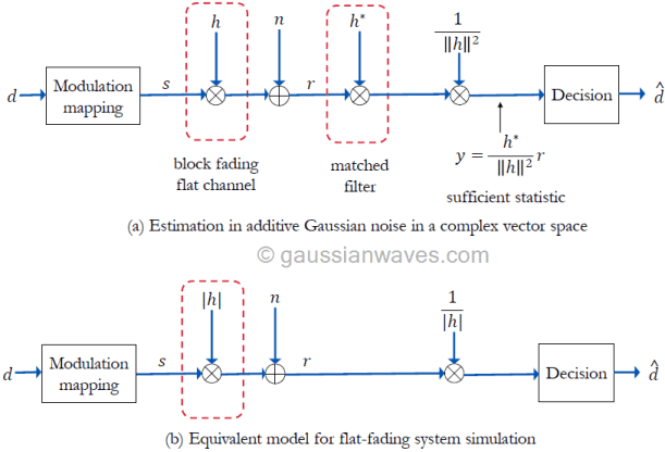
Figure 1: Simulation model for modulation and detection over flat fading channel
Simulation and performance results
In chapter 5 of the book Wireless communication systems in Matlab, the code implementation for complex baseband models for various digital modulators and demodulator are given. The computation and generation of AWGN noise is also given in the book. Using these models, we can create a unified simulation for code for simulating the performance of various modulation techniques over Rician flat-fading channel the simulation model shown in Figure 1(b).
An unified approach is employed to simulate the performance of any of the given modulation technique – MPSK, MQAM or MPAM. The simulation code (given in the book) will automatically choose the selected modulation type, performs Monte Carlo simulation, computes symbol error rates and plots them against the theoretical symbol error rate curves. The simulated performance results obtained for various modulations are shown in the Figure 2.
Figure 2: Performance of various modulations over Ricean flat fading channel
Rate this article: Note: There is a rating embedded within this post, please visit this post to rate it.
Key focus: Simulate bit error rate performance of Binary Phase Shift Keying (BPSK) modulation over AWGN channel using complex baseband equivalent model in Python & Matlab.
Why complex baseband equivalent model
The passband model and equivalent baseband model are fundamental models for simulating a communication system. In the passband model, also called as waveform simulation model, the transmitted signal, channel noise and the received signal are all represented by samples of waveforms. Since every detail of the RF carrier gets simulated, it consumes more memory and time.
In the case of discrete-time equivalent baseband model, only the value of a symbol at the symbol-sampling time instant is considered. Therefore, it consumes less memory and yields results in a very short span of time when compared to the passband models. Such models operate near zero frequency, suppressing the RF carrier and hence the number of samples required for simulation is greatly reduced. They are more suitable for performance analysis simulations. If the behavior of the system is well understood, the model can be simplified further.
In binary phase shift keying, all the information gets encoded in the phase of the carrier signal. The BPSK modulator accepts a series of information symbols drawn from the set m∈{0,1}, modulates them and transmits the modulated symbols over a channel.
The general expression for generating a M-PSK signal set is given by
Here, M denotes the modulation order and it defines the number of constellation points in the reference constellation. The value of M depends on the parameter k – the number of bits we wish to squeeze in a single M-PSK symbol. For example if we wish to squeeze in 3 bits (k=3) in one transmit symbol, then M = 2k = 23 = 8 and this results in 8-PSK configuration. M=2 gives BPSK (Binary Phase Shift Keying) configuration. The parameter A is the amplitude scaling factor, fc is the carrier frequency and g(t) is the pulse shape that satisfies orthonormal properties of basis functions.
Using trigonometric identity, equation (1) can be separated into cosine and sine basis functions as follows
Therefore, the signaling set {si,sq} or the constellation points for M-PSK modulation is given by,
For BPSK (M=2), the constellation points on the I-Q plane (Figure 1) are given by
In this simulation methodology, there is no need to simulate each and every sample of the BPSK waveform as per equation (1). Only the value of a symbol at the symbol-sampling time instant is considered. The steps for simulation of performance of BPSK over AWGN channel is as follows (Figure 2)
Generate a sequence of random bits of ones and zeros of certain length (Nsym typically set in the order of 10000)
Using the constellation points, map the bits to modulated symbols (For example, bit ‘0’ is mapped to amplitude value A, and bit ‘1’ is mapped to amplitude value -A)
Compute the total power in the sequence of modulated symbols and add noise for the given EbN0 (SNR) value (read this article on how to do this). The noise added symbols are the received symbols at the receiver.
Use thresholding technique, to detect the bits in the receiver. Based on the constellation diagram above, the detector at the receiver has to decide whether the receiver bit is above or below the threshold 0.
Compare the detected bits against the transmitted bits and compute the bit error rate (BER).
Figure 2: Simulation methodology for performance of BPSK modulation over AWGN channel
Let’s simulate the performance of BPSK over AWGN channel in Python & Matlab.
Simulation using Python
Following standalone code simulates the bit error rate performance of BPSK modulation over AWGN using Python version 3. The results are plotted in Figure 3.
Following code simulates the bit error rate performance of BPSK modulation over AWGN using basic installation of Matlab. You will need the add_awgn_noise function that was discussed in this article. The results will be same as Figure 3.
Minimum shift keying (MSK) is a special case of binary CPFSK with modulation index . It has features such as constant envelope, compact spectrum and good error rate performance. The fundamental problem with MSK is that the spectrum is not compact enough to satisfy the stringent requirements with respect to out-of-band radiation for technologies like GSM and DECT standard. These technologies have very high data rates approaching the RF channel bandwidth. A plot of MSK spectrum (Figure 1) will reveal that the sidelobes with significant energy, extend well beyond the transmission data rate. This is problematic, since it causes severe out-of-band interference in systems with closely spaced adjacent channels.
Minimum shift keying (MSK) is a special case of binary CPFSK with modulation index . It has features such as constant envelope, compact spectrum and good error rate performance. The fundamental problem with MSK is that the spectrum is not compact enough to satisfy the stringent requirements with respect to out-of-band radiation for technologies like GSM and DECT standard. These technologies have very high data rates approaching the RF channel bandwidth. A plot of MSK spectrum (Figure 1) will reveal that the sidelobes with significant energy, extend well beyond the transmission data rate. This is problematic, since it causes severe out-of-band interference in systems with closely spaced adjacent channels.
Figure 1: PSD estimates for BPSK, QPSK and MSK signals
To satisfy such requirements, the MSK spectrum can be easily manipulated by using a pre-modulation low pass filter (LPF). The pre-modulation LPF should have the following properties and it is found that a Gaussian LPF will satisfy all of them [1]
Sharp cut-off and narrow bandwidth – needed to suppress high frequency components.
Lower overshoot in the impulse response – providing protection against excessive instantaneous frequency deviations.
Preservation of filter output pulse area – thereby coherent detection can be applicable.
Pre-modulation Gaussian low pass filter
Gaussian Minimum Shift Keying (GMSK) is a modified MSK modulation technique, where the spectrum of MSK is manipulated by passing the rectangular shaped information pulses through a Gaussian LPF prior to the frequency modulation of the carrier. A typical Gaussian LPF, used in GMSK modulation standards, is defined by the zero-mean Gaussian (bell-shaped) impulse response.
The parameter is the 3-dB bandwidth of the LPF, which is determined from a parameter called as discussed next. If the input to the filter is an isolated unit rectangular pulse (), the response of the filter will be [2]
where,
It is important to note the distinction between the two equations – (1) and (2). The equation for defines the impulse response of the LPF, whereas the equation for , also called as frequency pulse shaping function, defines the LPF’s output when the filter gets excited with a rectangular pulse. This distinction is captured in Figure 2.
Figure 2: Gaussian LPF: Relating h(t) and g(t)
The aim of using GMSK modulation is to have a controlled MSK spectrum. Effectively, a variable parameter called , the product of 3-dB bandwidth of the LPF and the desired data-rate , is often used by the designers to control the amount of spectrum efficiency required for the desired application. As a consequence, the 3-dB bandwidth of the aforementioned LPF is controlled by the design parameter. The range for the parameter is given as . When , the impulse response becomes a Dirac delta function , resulting in a transparent LPF and hence this configuration corresponds to MSK modulation.
The Matlab function to implement the Gaussian LPF’s impulse response (equation (1)), is given in the book (For Python implementation, refer this book). The Gaussian impulse response is of infinite duration and hence in digital implementations it has to be defined for a finite interval, as dictated by the function argument in the code shown next. For example, in GSM standard, is chosen as 0.3 and the time truncation is done to three bit-intervals .
It is also necessary to normalize the filter coefficients of the computed LPF as
Based on the gaussianLPF Matlab function, given in the book (For Python implementation, refer this book), we can compute and plot the impulse response and the response to an isolated unit rectangular pulse – . The resulting plot is shown in Figure 3.
Binomial random variable, a discrete random variable, models the number of successes in mutually independent Bernoulli trials, each with success probability . The term Bernoulli trial implies that each trial is a random experiment with exactly two possible outcomes: success and failure. It can be used to model the total number of bit errors in the received data sequence of length that was transmitted over a binary symmetric channel of bit-error probability .
Generating binomial random sequence in Matlab
Let X denotes the total number of successes in mutually independent Bernoulli trials. For ease of understanding, let’s denote success as ‘1’ and failure as ‘0’. Suppose if a particular outcome of the experiment contains ones and zeros (example outcome: 1011101), the probability mass function↗ of is given by
A binomial random variable can be simulated by generating independent Bernoulli trials and summing up the results.
function X = binomialRV(n,p,L)
%Generate Binomial random number sequence
%n - the number of independent Bernoulli trials
%p - probability of success yielded by each trial
%L - length of sequence to generate
X = zeros(1,L);
for i=1:L,
   X(i) = sum(bernoulliRV(n,p));
end
end
Following program demonstrates how to generate a sequence of binomially distributed random numbers, plot the estimated and theoretical probability mass functions for the chosen parameters (Figure 1).
n=30; p=1/6; %number of trails and success probability
X = binomialRV(n,p,10000);%generate 10000 bino rand numbers
X_pdf = pdf('Binomial',0:n,n,p); %theoretical probility density
histogram(X,'Normalization','pdf'); %plot histogram
hold on; plot(0:n,X_pdf,'r'); %plot computed theoreical PDF
Figure 1: PMF generated from binomial random variable for three different cases of n and p
PMF sums to unity
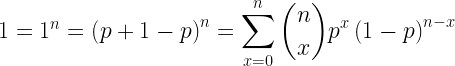
Let’s verify theoretically, the fact that the PMF of the binomial distribution sums to unity. Using the result of Binomial theorem↗,
Mean and variance
The mean number of success in a binomial distribution is
The variance is
Rate this article: Note: There is a rating embedded within this post, please visit this post to rate it.
Bernoulli random variable is a discrete random variable with two outcomes – success and failure, with probabilities p and (1-p). It is a good model for binary data generators and also for modeling bit error patterns in the received binary data when a communication channel introduces random errors.
To generate a Bernoulli random variable X, in which the probability of success P(X=1)=p for some p ϵ (0,1), the discrete inverse transform method [1] can be applied on the continuous uniform random variable U(0,1) using the steps below.
● Generate uniform random number U in the interval (0,1) ● If U<p, set X=1, else set X=0
#bernoulliRV.m: Generating Bernoulli random number with success probability p
function X = bernoulliRV(L,p)
%Generate Bernoulli random number with success probability p
%L is the length of the sequence generated
U = rand(1,L); %continuous uniform random numbers in (0,1)
X = (U<p); end
Verifying law of large numbers
In probability theory, the law of large numbers is a theorem that involves repeating an experiment for a large number of times. According to this law, as the number of trials tend to become large, the average result obtained will be close to the expected value.
Let’s toss a coin with probability of heads . This experiment is repeated for a large number of times, say and the average result for each trial are calculated in a cumulative fashion.
#lawOfLargeNumbers.m: Law of large numbers illustrated using Bernoulli random variable
n=1000; %number of trials
p=0.7; %probability of success
X=bernoulliRV(n,p); %Bernoulli random variable
y_sum=sum(triu(repmat(X,[prod(size(X)) 1])')); %cumulative sum
avg = y_sum./(1:1:n); %average of results
plot(1:1:n,avg,'.'); hold on;
xlabel('Trial #'); ylabel('Probability of Heads');
plot(p*ones(1,n),'r'); legend('average','expected');
In coherent detection, the receiver derives its demodulation frequency and phase references using a carrier synchronization loop. Such synchronization circuits may introduce phase ambiguity in the detected phase, which could lead to erroneous decisions in the demodulated bits. For example, Costas loop exhibits phase ambiguity of integral multiples of radians at the lock-in points. As a consequence, the carrier recovery may lock in radians out-of-phase thereby leading to a situation where all the detected bits are completely inverted when compared to the bits during perfect carrier synchronization. Phase ambiguity can be efficiently combated by applying differential encoding at the BPSK modulator input (Figure 1) and by performing differential decoding at the output of the coherent demodulator at the receiver side (Figure 2).
In ordinary BPSK transmission, the information is encoded as absolute phases: for binary 1 and for binary 0. With differential encoding, the information is encoded as the phase difference between two successive samples. Assuming is the message bit intended for transmission, the differential encoded output is given as
The differentially encoded bits are then BPSK modulated and transmitted. On the receiver side, the BPSK sequence is coherently detected and then decoded using a differential decoder. The differential decoding is mathematically represented as
This method can deal with the phase ambiguity introduced by synchronization circuits. However, it suffers from performance penalty due to the fact that the differential decoding produces wrong bits when: a) the preceding bit is in error and the present bit is not in error , or b) when the preceding bit is not in error and the present bit is in error. After differential decoding, the average bit error rate of coherently detected BPSK over AWGN channel is given by
Figure 2: Coherent detection of differentially encoded BPSK signal
Following is the Matlab implementation of the waveform simulation model for the method discussed above. Both the differential encoding and differential decoding blocks, illustrated in Figures 1 and 2, are linear time-invariant filters. The differential encoder is realized using IIR type digital filter and the differential decoder is realized as FIR filter.
File 1: dbpsk_coherent_detection.m: Coherent detection of D-BPSK over AWGN channel
Figure 3 shows the simulated BER points together with the theoretical BER curves for differentially encoded BPSK and the conventional coherently detected BPSK system over AWGN channel.
Key focus: Demodulation of phase modulated signal by extracting instantaneous phase can be done using Hilbert transform. Hands-on demo in Python & Matlab.
Phase modulated signal:
The concept of instantaneous amplitude/phase/frequency are fundamental to information communication and appears in many signal processing application. We know that a monochromatic signal of form x(t) = a cos(ω t + ɸ) cannot carry any information. To carry information, the signal need to be modulated. Different types of modulations can be performed – amplitude modulation, phase modulation / frequency modulation.
In amplitude modulation, the information is encoded as variations in the amplitude of a carrier signal. Demodulation of an amplitude modulated signal, involves extraction of envelope of the modulated signal. This was discussed and demonstrated here.
In phase modulation, the information is encoded as variations in the phase of the carrier signal. In its generic form, a phase modulated signal is expressed as an information-bearing sinusoidal signal modulating another sinusoidal carrier signal
\[x(t) = A cos \left[ 2 \pi f_c t + \beta + \alpha sin \left( 2 \pi f_m t + \theta \right) \right] \quad \quad \quad (1)\]
where, m(t) = α sin (2 π fm t + θ ) represents the information-bearing modulating signal, with the following parameters
α – amplitude of the modulating sinusoidal signal fm – frequency of the modulating sinusoidal signal θ – phase offset of the modulating sinusoidal signal
The carrier signal has the following parameters
A – amplitude of the carrier fc – frequency of the carrier and fc>>fm β – phase offset of the carrier
Demodulating a phase modulated signal:
The phase modulated signal shown in equation (1), can be simply expressed as
\[x(t) = A cos \left[ \phi(t) \right] \quad\quad\quad (2) \]
Here, ɸ(t) is the instantaneous phase that varies according to the information signal m(t).
A phase modulated signal of form x(t) can be demodulated by forming an analytic signal by applying Hilbert transform and then extracting the instantaneous phase. This method is explained here.
We note that the instantaneous phase is ɸ(t) = 2 π fc t + β + α sin (2 π fm t + θ) is linear in time, that is proportional to 2 π fc t . This linear offset needs to be subtracted from the instantaneous phase to obtained the information bearing modulated signal. If the carrier frequency is known at the receiver, this can be done easily. If not, the carrier frequency term 2 π fc t needs to be estimated using a linear fitof the unwrapped instantaneous phase. The following Matlab and Python codes demonstrate all these methods.
Matlab code
%Demonstrate simple Phase Demodulation using Hilbert transform
clearvars; clc;
fc = 240; %carrier frequency
fm = 10; %frequency of modulating signal
alpha = 1; %amplitude of modulating signal
theta = pi/4; %phase offset of modulating signal
beta = pi/5; %constant carrier phase offset
receiverKnowsCarrier= 'False'; %If receiver knows the carrier frequency & phase offset

fs = 8*fc; %sampling frequency
duration = 0.5; %duration of the signal
t = 0:1/fs:1-1/fs; %time base

%Phase Modulation
m_t = alpha*sin(2*pi*fm*t + theta); %modulating signal
x = cos(2*pi*fc*t + beta + m_t ); %modulated signal

figure(); subplot(2,1,1)
plot(t,m_t) %plot modulating signal
title('Modulating signal'); xlabel('t'); ylabel('m(t)')

subplot(2,1,2)
plot(t,x) %plot modulated signal
title('Modulated signal'); xlabel('t');ylabel('x(t)')

%Add AWGN noise to the transmitted signal
nMean = 0; %noise mean
nSigma = 0.1; %noise sigma
n = nMean + nSigma*randn(size(t)); %awgn noise
r = x + n;  %noisy received signal

%Demodulation of the noisy Phase Modulated signal
z= hilbert(r); %form the analytical signal from the received vector
inst_phase = unwrap(angle(z)); %instaneous phase

%If receiver don't know the carrier, estimate the subtraction term
if strcmpi(receiverKnowsCarrier,'True')
    offsetTerm = 2*pi*fc*t+beta; %if carrier frequency & phase offset is known
else
    p = polyfit(t,inst_phase,1); %linearly fit the instaneous phase
    estimated = polyval(p,t); %re-evaluate the offset term using the fitted values
    offsetTerm = estimated;
end

demodulated = inst_phase - offsetTerm;

figure()
plot(t,demodulated); %demodulated signal
title('Demodulated signal'); xlabel('n'); ylabel('\hat{m(t)}');
Python code
import numpy as np
from scipy.signal import hilbert
import matplotlib.pyplot as plt
PI = np.pi

fc = 240 #carrier frequency
fm = 10 #frequency of modulating signal
alpha = 1 #amplitude of modulating signal
theta = PI/4 #phase offset of modulating signal
beta = PI/5 #constant carrier phase offset
receiverKnowsCarrier= False; #If receiver knows the carrier frequency & phase offset

fs = 8*fc #sampling frequency
duration = 0.5 #duration of the signal
t = np.arange(int(fs*duration)) / fs #time base

#Phase Modulation
m_t = alpha*np.sin(2*PI*fm*t + theta) #modulating signal
x = np.cos(2*PI*fc*t + beta + m_t ) #modulated signal

plt.figure()
plt.subplot(2,1,1)
plt.plot(t,m_t) #plot modulating signal
plt.title('Modulating signal')
plt.xlabel('t')
plt.ylabel('m(t)')
plt.subplot(2,1,2)
plt.plot(t,x) #plot modulated signal
plt.title('Modulated signal')
plt.xlabel('t')
plt.ylabel('x(t)')

#Add AWGN noise to the transmitted signal
nMean = 0 #noise mean
nSigma = 0.1 #noise sigma
n = np.random.normal(nMean, nSigma, len(t))
r = x + n  #noisy received signal

#Demodulation of the noisy Phase Modulated signal
z= hilbert(r) #form the analytical signal from the received vector
inst_phase = np.unwrap(np.angle(z))#instaneous phase

#If receiver don't know the carrier, estimate the subtraction term
if receiverKnowsCarrier:
    offsetTerm = 2*PI*fc*t+beta; #if carrier frequency & phase offset is known
else:
    p = np.poly1d(np.polyfit(t,inst_phase,1)) #linearly fit the instaneous phase
    estimated = p(t) #re-evaluate the offset term using the fitted values
    offsetTerm = estimated

demodulated = inst_phase - offsetTerm

plt.figure()
plt.plot(t,demodulated) #demodulated signal
plt.title('Demodulated signal')
plt.xlabel('n')
plt.ylabel('\hat{m(t)}')
Results
Figure 1: Phase modulation – modulating signal and modulated (transmitted) signal
Key focus: Learn how to use Hilbert transform to extract envelope, instantaneous phase and frequency from a modulated signal. Hands-on demo using Python & Matlab.
The concept of instantaneous amplitude/phase/frequency are fundamental to information communication and appears in many signal processing application. We know that a monochromatic signal of form cannot carry any information. To carry information, the signal need to be modulated. Take for example the case of amplitude modulation, in which a positive real-valued signal modulates a carrier . That is, the amplitude modulation is effected by multiplying the information bearing signal with the carrier signal .
Here, is the angular frequency of the signal measured in radians/sec and is related to the temporal frequency as . The term is also called instantaneous amplitude.
Similarly, in the case of phase or frequency modulations, the concept of instantaneous phase or instantaneous frequency is required for describing the modulated signal.
Here, is the constant amplitude factor (no change in the envelope of the signal) and is the instantaneous phase which varies according to the information. The instantaneous angular frequency is expressed as the derivative of instantaneous phase.
Generalizing these concepts, if a signal is expressed as
The instantaneous amplitude or the envelope of the signal is given by
The instantaneous phase is given by
The instantaneous angular frequency is derived as
The instantaneous temporal frequency is derived as
Problem statement
An amplitude modulated signal is formed by multiplying a sinusoidal information and a linear frequency chirp. The information content is expressed as and the linear frequency chirp is made to vary from to . Given the modulated signal, extract the instantaneous amplitude (envelope), instantaneous phase and the instantaneous frequency.
Solution
We note that the modulated signal is a real-valued signal. We also take note of the fact that amplitude/phase and frequency can be easily computed if the signal is expressed in complex form. Which transform should we use such that the we can convert a real signal to the complex plane without altering the required properties ?? Answer: Apply Hilbert transform and form the analytic signal on the complex plane. Figure 1 illustrates this concept.
Figure 1: Converting a real-valued signal to complex plane using Hilbert Transform
If we express the real-valued modulated signal as an analytic signal, it is expressed in complex plane as
where, (HT[.]) represents the Hilbert Transform operation. Now, the required parameters are very easy to obtain.
The instantaneous amplitude (envelope extraction) is computed in the complex plane as
The instantaneous phase is computed in the complex plane as
The instantaneous temporal frequency is computed in the complex plane as
Once we know the instantaneous phase, the carrier can be regenerated as . The regenerated carrier is often referred as Temporal Fine Structure (TFS) in Acoustic signal processing [1].
Matlab
fs = 600; %sampling frequency in Hz
t = 0:1/fs:1-1/fs; %time base
a_t = 1.0 + 0.7 * sin(2.0*pi*3.0*t) ; %information signal
c_t = chirp(t,20,t(end),80); %chirp carrier
x = a_t .* c_t; %modulated signal

subplot(2,1,1); plot(x);hold on; %plot the modulated signal

z = hilbert(x); %form the analytical signal
inst_amplitude = abs(z); %envelope extraction
inst_phase = unwrap(angle(z));%inst phase
inst_freq = diff(inst_phase)/(2*pi)*fs;%inst frequency

%Regenerate the carrier from the instantaneous phase
regenerated_carrier = cos(inst_phase);

plot(inst_amplitude,'r'); %overlay the extracted envelope
title('Modulated signal and extracted envelope'); xlabel('n'); ylabel('x(t) and |z(t)|');
subplot(2,1,2); plot(cos(inst_phase));
title('Extracted carrier or TFS'); xlabel('n'); ylabel('cos[\omega(t)]');
Python
import numpy as np
from scipy.signal import hilbert, chirp
import matplotlib.pyplot as plt

fs = 600.0 #sampling frequency
duration = 1.0 #duration of the signal
t = np.arange(int(fs*duration)) / fs #time base

a_t =  1.0 + 0.7 * np.sin(2.0*np.pi*3.0*t)#information signal
c_t = chirp(t, 20.0, t[-1], 80) #chirp carrier
x = a_t * c_t #modulated signal

plt.subplot(2,1,1)
plt.plot(x) #plot the modulated signal

z= hilbert(x) #form the analytical signal
inst_amplitude = np.abs(z) #envelope extraction
inst_phase = np.unwrap(np.angle(z))#inst phase
inst_freq = np.diff(inst_phase)/(2*np.pi)*fs #inst frequency

#Regenerate the carrier from the instantaneous phase
regenerated_carrier = np.cos(inst_phase)

plt.plot(inst_amplitude,'r'); #overlay the extracted envelope
plt.title('Modulated signal and extracted envelope')
plt.xlabel('n')
plt.ylabel('x(t) and |z(t)|')
plt.subplot(2,1,2)
plt.plot(regenerated_carrier)
plt.title('Extracted carrier or TFS')
plt.xlabel('n')
plt.ylabel('cos[\omega(t)]')
Key focus of this article: Understand the relationship between analytic signal, Hilbert transform and FFT. Hands-on demonstration using Python and Matlab.
Introduction
Fourier Transform of a real-valued signal is complex-symmetric. It implies that the content at negative frequencies are redundant with respect to the positive frequencies. In their works, Gabor [1]and Ville [2], aimed to create an analytic signal by removing redundant negative frequency content resulting from the Fourier transform. The analytic signal is complex-valued but its spectrum will be one-sided (only positive frequencies) that preserved the spectral content of the original real-valued signal. Using an analytic signal instead of the original real-valued signal, has proven to be useful in many signal processing applications. For example, in spectral analysis, use of analytic signal in-lieu of the original real-valued signal mitigates estimation biases and eliminates cross-term artifacts due to negative and positive frequency components [3].
Let be a real-valued non-bandlimited finite energy signal, for which we wish to construct a corresponding analytic signal . The Continuous Time Fourier Transform of is given by
Lets say the magnitude spectrum of is as shown in Figure 1(a). We note that the signal is a real-valued and its magnitude spectrum is symmetric and extends infinitely in the frequency domain.
Figure 1: (a) Spectrum of continuous signal x(t) and (b) spectrum of analytic signal z(t)
As mentioned in the introduction, an analytic signal can be formed by suppressing the negative frequency contents of the Fourier Transform of the real-valued signal. That is, in frequency domain, the spectral content of the analytic signal is given by
The corresponding spectrum of the resulting analytic signal is shown in Figure 1(b).
Since the spectrum of the analytic signal is one-sided, the analytic signal will be complex valued in the time domain, hence the analytic signal can be represented in terms of real and imaginary components as . Since the spectral content is preserved in an analytic signal, it turns out that the real part of the analytic signal in time domain is essentially the original real-valued signal itself . Then, what takes place of the imaginary part ? Who is the companion to x(t) that occupies the imaginary part in the resulting analytic signal ? Summarizing as equation,
It is interesting to note that Hilbert transform [4]can be used to find a companion function (imaginary part in the equation above) to a real-valued signal such that the real signal can be analytically extended from the real axis to the upper half of the complex plane . Denoting Hilbert transform as , the analytic signal is given by
From these discussion, we can see that an analytic signal for a real-valued signal , can be constructed using two approaches.
● Frequency domain approach: The one-sided spectrum of is formed from the two-sided spectrum of the real-valued signal by applying equation (2) ● Time domain approach: Using Hilbert transform approach given in equation (4)
One of the important property of an analytic signal is that its real and imaginary components are orthogonal
Discrete-time analytic signal
Since we are in digital era, we are more interested in discrete-time signal processing. Consider a continuous real-valued signal gets sampled at interval seconds and results in real-valued discrete samples , i.e, . The spectrum of the continuous signal is shown in Figure 2(a). The spectrum of that results from the process of periodic sampling is given in Figure 2(b) (Refer here more details on the process of sampling). The spectrum of discrete-time signal can be obtained by Discrete-Time Fourier Transform (DTFT).
Figure 2: (a) CTFT of continuous signal x(t), (b) Spectrum of x[n] resulted due to periodic sampling and (c) Periodic one-sided spectrum of analytical signal z[n]
At this point, we would like to construct a discrete-time analytic signal from the real-valued sampled signal . We wish the analytic signal is complex valued and should satisfy the following two desired properties
● The real part of the analytic signal should be same as the original real-valued signal. ● The real and imaginary part of the analytic signal should satisfy the following property of orthogonality
In Frequency domain approach for the continuous-time case, we saw that an analytic signal is constructed by suppressing the negative frequency components from the spectrum of the real signal. We cannot do this for our periodically sampled signal . Periodic mirroring nature of the spectrum prevents one from suppressing the negative components. If we do so, it will vanish the entire spectrum. One solution to this problem is to set the negative half of each spectral period to zero. The resulting spectrum of the analytic signal is shown in Figure 2(c).
Given a record of samples of even length , the procedure to construct the analytic signal is as follows. This method satisfies both the desired properties listed above.
● Compute the -point DTFT of using FFT ● N-point periodic one-sided analytic signal is computed by the following transform
● Finally, the analytic signal (z[n]) is obtained by taking the inverse DTFT of
Matlab
The given procedure can be coded in Matlab using the FFT function. Given a record of real-valued samples , the corresponding analytic signal can be constructed as given next. Note that the Matlab has an inbuilt function to compute the analytic signal. The in-built function is called hilbert.
function z = analytic_signal(x)
%x is a real-valued record of length N, where N is even %returns the analytic signal z[n]
x = x(:); %serialize
N = length(x);
X = fft(x,N);
z = ifft([X(1); 2*X(2:N/2); X(N/2+1); zeros(N/2-1,1)],N);
end
To test this function, we create a 5 seconds record of a real-valued sine signal. The analytic signal is constructed and the orthogonal components are plotted in Figure 3. From the plot, we can see that the real part of the analytic signal is exactly same as the original signal (which is the cosine signal) and the imaginary part of the analytic signal is phase shifted version of the original signal. We note that the imaginary part of the analytic signal is a cosine function with amplitude scaled by which is none other than the Hilbert transform of sine function.
t=0:0.001:0.5-0.001;
x = sin(2*pi*10*t); %real-valued f = 10 Hz
subplot(2,1,1); plot(t,x);%plot the original signal
title('x[n] - original signal'); xlabel('n'); ylabel('x[n]');

z = analytic_signal(x); %construct analytic signal
subplot(2,1,2); plot(t, real(z), 'k'); hold on;
plot(t, imag(z), 'r');
title('Components of Analytic signal');
xlabel('n'); ylabel('z_r[n] and z_i[n]');
legend('Real(z[n])','Imag(z[n])');
Python
Equivalent code in Python is given below (tested with Python 3.6.0)
import numpy as np
def main():
    t = np.arange(start=0,stop=0.5,step=0.001)
    x = np.sin(2*np.pi*10*t)

    import matplotlib.pyplot as plt
    plt.subplot(2,1,1)
    plt.plot(t,x)
    plt.title('x[n] - original signal')
    plt.xlabel('n')
    plt.ylabel('x[n]')

    z = analytic_signal(x)

    plt.subplot(2,1,2)
    plt.plot(t,z.real,'k',label='Real(z[n])')
    plt.plot(t,z.imag,'r',label='Imag(z[n])')
    plt.title('Components of Analytic signal')
    plt.xlabel('n')
    plt.ylabel('z_r[n] and z_i[n]')
    plt.legend()

def analytic_signal(x):
    from scipy.fftpack import fft,ifft
    N = len(x)
    X = fft(x,N)
    h = np.zeros(N)
    h[0] = 1
    h[1:N//2] = 2*np.ones(N//2-1)
    h[N//2] = 1
    Z = X*h
    z = ifft(Z,N)
    return z

if __name__ == '__main__':
    main()
We should note that the hilbert function in Matlab returns the analytic signal $latex z[n]$ not the hilbert transform of the signal. To get the hilbert transform, we should simply get the imaginary part of the analytic signal. Since we have written our own function to compute the analytic signal, getting the hilbert transform of a real-valued signal goes like this.
Synopsis: Cyclic prefix in OFDM, tricks a natural channel to perform circular convolution. This simplifies equalizer design at the receiver. Hands-on demo in Matlab.
Cyclic Prefix-ed OFDM
A cyclic-prefixed OFDM(CP-OFDM) transceiver architecture is typically implemented using inverse discrete Fourier transform (IDFT) and discrete Fourier transform (DFT) blocks (refer Figure 13.3). In an OFDM transmitter, the modulated symbols are assigned to individual subcarriers and sent to an IDFT block. The output of the IDFT block, generally viewed as time domain samples, results in an OFDM symbol. Such OFDM symbols are then transmitted across a channel with certain channel impulse response (CIR). On the other hand, the receiver applies DFT over the received OFDM symbols for further demodulation of the information in the individual subcarriers.
In reality, a multipath channel or any channel in nature acts as a linear filter on the transmitted OFDM symbols. Mathematically, the transmitted OFDM symbol (denoted as gets linearly convolved with the CIR and gets corrupted with additive white gaussian noise – designated as . Denoting linear convolution as ‘‘, the received signal in discrete-time can be represented as
The idea behind using OFDM is to combat frequency selective fading, where different frequency components of a transmitted signal can undergo different levels of fading. The OFDM divides the available spectrum in to small chunks called sub-channels. Within the subchannels, the fading experienced by the individual modulated symbol can be considered flat. This opens-up the possibility of using a simple frequency domain equalizer to neutralize the channel effects in the individual subchannels.
Circular convolution and designing a simple frequency domain equalizer
From one of the DFT properties, we know that the circular convolution of two sequences in time domain is equivalent to the multiplication of their individual responses in frequency domain.
Let and are two sequences of length with their DFTs denoted as and respectively. Denoting circular convolution as ,
If we ignore channel noise in the OFDM transmission, the received signal is written as
We can note that the channel performs a linear convolution operation on the transmitted signal. Instead, if the channel performs circular convolution (which is not the case in nature) then the equation would have been
By applying the DFT property given in equation 2,
As a consequence, the channel effects can be neutralized at the receiver using a simple frequency domain equalizer (actually this is a zero-forcing equalizer when viewed in time domain) that just inverts the estimated channel response and multiplies it with the frequency response of the received signal to obtain the estimates of the OFDM symbols in the subcarriers as
Demonstrating the role of Cyclic Prefix
The simple frequency domain equalizer shown in equation 6 is possible only if the channel performs circular convolution. But in nature, all channels perform linear convolution. The linear convolution can be converted into circular convolution by adding Cyclic Prefix (CP) in the OFDM architecture. The addition of CP makes the linear convolution imparted by the channel appear as circular convolution to the DFT process at the receiver (Reference [1]).
Let’s understand this by demonstration.
To simply stuffs, we will create two randomized vectors for and . is of length , the channel impulse response is of length and we intend to use -point DFT/IDFT wherever applicable.
N=8; %period of DFT
s = randn(1,8);
h = randn(1,3);
>> s =   -0.0155    2.5770    1.9238   -0.0629   -0.8105    0.6727   -1.5924   -0.8007
>> h =   -0.4878   -1.5351    0.2355
Now, convolve the vectors and linearly and circularly. The outputs are plotted in Figure 1. We note that the linear convolution and the circular convolution does not yield identical results.
lin_s_h = conv(h,s) %linear convolution of h and s
cir_s_h = cconv(h,s,N) % circular convolution of h and s with period N
Figure 1: Difference between linear convolution and circular convolution
Let’s append a cyclic prefix to the signal by copying last symbols from and pasting it to its front. Since the channel delay is 3 symbols (CIR of length 3), we need to add atleast 2 CP symbols.
Ncp = 2; %number of symbols to copy and paste for CP
s_cp = [s(end-Ncp+1:end) s]; %copy last Ncp symbols from s and prefix it.
Compare the outputs due to cir_s_h and lin_scp_h. We can immediately recognize that that the middle section of lin_scp_h is exactly same as the cir_s_h vector. This is shown in the figure 2.
We have just tricked the channel to perform circular convolution by adding a cyclic extension to the OFDM symbol. At the receiver, we are only interested in the middle section of the lin_scp_h which is the channel output. The first block in the OFDM receiver removes the additional symbols from the front and back of the channel output. The resultant vector is the received symbol r after the removal of cyclic prefix in the receiver.
r = lin_scp_h(Ncp+1:N+Ncp)%cut from index Ncp+1 to N+Ncp
Verifying DFT property
The DFT property given in equation 5 can be re-written as
To verify this in Matlab, take N-point DFTs of the received signal and CIR. Then, we can see that the IDFT of product of DFTs of and will be equal to the N-point circular convolution of and
R = fft(r,N); %frequency response of received signal
H = fft(h,N); %frequency response of CIR
S = fft(s,N); %frequency response of OFDM signal (non CP)

r1 = ifft(S.*H); %IFFT of product of individual DFTs

display(['IFFT(DFT(H)*DFT(S)) : ',num2str(r1)])
display([cconv(s,h): ', numstr(r)])
This website uses cookies to improve your experience while you navigate through the website. Out of these, the cookies that are categorized as necessary are stored on your browser as they are essential for the working of basic functionalities of the website. We also use third-party cookies that help us analyze and understand how you use this website. These cookies will be stored in your browser only with your consent. You also have the option to opt-out of these cookies. But opting out of some of these cookies may affect your browsing experience.
Necessary cookies are absolutely essential for the website to function properly. These cookies ensure basic functionalities and security features of the website, anonymously.
Cookie
Duration
Description
cookielawinfo-checbox-analytics
11 months
This cookie is set by GDPR Cookie Consent plugin. The cookie is used to store the user consent for the cookies in the category "Analytics".
cookielawinfo-checbox-analytics
11 months
This cookie is set by GDPR Cookie Consent plugin. The cookie is used to store the user consent for the cookies in the category "Analytics".
cookielawinfo-checbox-functional
11 months
The cookie is set by GDPR cookie consent to record the user consent for the cookies in the category "Functional".
cookielawinfo-checbox-functional
11 months
The cookie is set by GDPR cookie consent to record the user consent for the cookies in the category "Functional".
cookielawinfo-checbox-others
11 months
This cookie is set by GDPR Cookie Consent plugin. The cookie is used to store the user consent for the cookies in the category "Other.
cookielawinfo-checbox-others
11 months
This cookie is set by GDPR Cookie Consent plugin. The cookie is used to store the user consent for the cookies in the category "Other.
cookielawinfo-checkbox-necessary
11 months
This cookie is set by GDPR Cookie Consent plugin. The cookies is used to store the user consent for the cookies in the category "Necessary".
cookielawinfo-checkbox-performance
11 months
This cookie is set by GDPR Cookie Consent plugin. The cookie is used to store the user consent for the cookies in the category "Performance".
viewed_cookie_policy
11 months
The cookie is set by the GDPR Cookie Consent plugin and is used to store whether or not user has consented to the use of cookies. It does not store any personal data.
Functional cookies help to perform certain functionalities like sharing the content of the website on social media platforms, collect feedbacks, and other third-party features.
Performance cookies are used to understand and analyze the key performance indexes of the website which helps in delivering a better user experience for the visitors.
Analytical cookies are used to understand how visitors interact with the website. These cookies help provide information on metrics the number of visitors, bounce rate, traffic source, etc.


![\mu = E[X] = np](https://s0.wp.com/latex.php?latex=%5Cmu+%3D+E%5BX%5D+%3D+np+&bg=ffffff&fg=000&s=2&c=20201002)

![\sigma^2 = E\left[ \left(X - \mu \right)^2 \right] = np (1-p)](https://s0.wp.com/latex.php?latex=%5Csigma%5E2+%3D+E%5Cleft%5B+%5Cleft%28X+-+%5Cmu+%5Cright%29%5E2+%5Cright%5D+%3D+np+%281-p%29+&bg=ffffff&fg=000&s=2&c=20201002)


![a[k]](https://s0.wp.com/latex.php?latex=a%5Bk%5D&bg=ffffff&fg=000&s=0&c=20201002)

![b[k] = b[k-1] \oplus a[k] \;\;\;\;\;\; (modulo-2) \;\;\;\;\;\; (1)](https://s0.wp.com/latex.php?latex=b%5Bk%5D+%3D+b%5Bk-1%5D+%5Coplus+a%5Bk%5D+%5C%3B%5C%3B%5C%3B%5C%3B%5C%3B%5C%3B+%28modulo-2%29+%5C%3B%5C%3B%5C%3B%5C%3B%5C%3B%5C%3B+%281%29+&bg=ffffff&fg=000&s=2&c=20201002)

![a[k] = b[k] \oplus b[k-1] \;\;\;\;\;\; (modulo-2) \;\;\;\;\;\; (2)](https://s0.wp.com/latex.php?latex=a%5Bk%5D+%3D+b%5Bk%5D+%5Coplus+b%5Bk-1%5D%C2%A0+%5C%3B%5C%3B%5C%3B%5C%3B%5C%3B%5C%3B+%28modulo-2%29+%5C%3B%5C%3B%5C%3B%5C%3B%5C%3B%5C%3B+%282%29+&bg=ffffff&fg=000&s=2&c=20201002)


![P_b = erfc \left(\sqrt{\frac{E_b}{N_0}} \right) \left[ 1-\frac{1}{2} erfc \left( \sqrt{\frac{E_b}{N_0}} \right) \right] \;\; (3)](https://s0.wp.com/latex.php?latex=P_b+%3D+erfc+%5Cleft%28%5Csqrt%7B%5Cfrac%7BE_b%7D%7BN_0%7D%7D+%5Cright%29+%5Cleft%5B+1-%5Cfrac%7B1%7D%7B2%7D+erfc+%5Cleft%28+%5Csqrt%7B%5Cfrac%7BE_b%7D%7BN_0%7D%7D+%5Cright%29+%5Cright%5D+%5C%3B%5C%3B+%283%29+&bg=ffffff&fg=000&s=2&c=20201002)


![x(t) = a(t) cos \left[ \phi (t) \right]](https://s0.wp.com/latex.php?latex=x%28t%29+%3D+a%28t%29+cos+%5Cleft%5B+%5Cphi+%28t%29+%5Cright%5D+&bg=ffffff&fg=000&s=0&c=20201002)


![z(t) = z_r(t) + j z_i(t) = x(t) + j HT \left[ x(t) \right]](https://s0.wp.com/latex.php?latex=z%28t%29+%3D+z_r%28t%29+%2B+j+z_i%28t%29+%3D+x%28t%29+%2B+j+HT+%5Cleft%5B+x%28t%29+%5Cright%5D+&bg=ffffff&fg=000&s=2&c=20201002)


![\phi(t) = \angle z(t) = arctan \left[ \frac{z_i(t)}{z_r(t)} \right]](https://s0.wp.com/latex.php?latex=%5Cphi%28t%29+%3D+%5Cangle+z%28t%29+%3D+arctan+%5Cleft%5B+%5Cfrac%7Bz_i%28t%29%7D%7Bz_r%28t%29%7D+%5Cright%5D+&bg=ffffff&fg=000&s=2&c=20201002)


![cos[\phi(t)]](https://s0.wp.com/latex.php?latex=cos%5B%5Cphi%28t%29%5D&bg=ffffff&fg=000&s=0&c=20201002)


![x[n]](https://s0.wp.com/latex.php?latex=x%5Bn%5D&bg=ffffff&fg=000&s=0&c=20201002)
![x[n] = x(nT)](https://s0.wp.com/latex.php?latex=x%5Bn%5D+%3D+x%28nT%29+&bg=ffffff&fg=000&s=0&c=20201002)

![X(f) = \displaystyle{ T \sum_{n=0}^{N-1} x[n] e^{-j 2 \pi f n T} }\quad (6)](https://s0.wp.com/latex.php?latex=X%28f%29+%3D+%5Cdisplaystyle%7B+T+%5Csum_%7Bn%3D0%7D%5E%7BN-1%7D+x%5Bn%5D+e%5E%7B-j+2+%5Cpi+f+n+T%7D+%7D%5Cquad+%286%29+%C2%A0&bg=ffffff&fg=000&s=2&c=20201002)

![(a) CTFT of continuous signal x(t), (b) Spectrum of x[n] resulted due to periodic sampling and (c) Periodic one-sided spectrum of analytical signal z[n]](https://i0.wp.com/www.gaussianwaves.com/gaussianwaves/wp-content/uploads/2017/04/discrete_time_analytic_signal_PNG.png?resize=594%2C494&ssl=1)
![z[n]](https://s0.wp.com/latex.php?latex=z%5Bn%5D&bg=ffffff&fg=000&s=0&c=20201002)
![z[n] = z_r[n] + j z_i[n]](https://s0.wp.com/latex.php?latex=z%5Bn%5D+%3D+z_r%5Bn%5D+%2B+j+z_i%5Bn%5D&bg=ffffff&fg=000&s=0&c=20201002)

![z_r[n] = x[n]](https://s0.wp.com/latex.php?latex=z_r%5Bn%5D+%3D+x%5Bn%5D&bg=ffffff&fg=000&s=0&c=20201002)

![\displaystyle{ \sum_{n=0}^{N-1} z_r[n] z_i[n] = 0 }](https://s0.wp.com/latex.php?latex=%5Cdisplaystyle%7B+%5Csum_%7Bn%3D0%7D%5E%7BN-1%7D+z_r%5Bn%5D+z_i%5Bn%5D+%3D+0+%7D++&bg=ffffff&fg=000&s=2&c=20201002)


![Z[m]](https://s0.wp.com/latex.php?latex=Z%5Bm%5D&bg=ffffff&fg=000&s=0&c=20201002)

![z[n] = \displaystyle{ \frac{1}{NT} \sum_{m=0}^{N-1} z[m] \; exp \left( j 2 \pi mn/N\right)}](https://s0.wp.com/latex.php?latex=z%5Bn%5D+%3D+%5Cdisplaystyle%7B+%5Cfrac%7B1%7D%7BNT%7D+%5Csum_%7Bm%3D0%7D%5E%7BN-1%7D+z%5Bm%5D+%5C%3B+exp+%5Cleft%28+j+2+%5Cpi+mn%2FN%5Cright%29%7D+&bg=ffffff&fg=000&s=2&c=20201002)


![s[n]](https://s0.wp.com/latex.php?latex=s%5Bn%5D&bg=ffffff&fg=000&s=0&c=20201002)
![h[n]](https://s0.wp.com/latex.php?latex=h%5Bn%5D&bg=ffffff&fg=000&s=0&c=20201002)

![w[n]](https://s0.wp.com/latex.php?latex=w%5Bn%5D&bg=ffffff&fg=000&s=0&c=20201002)


![r[n] = h[n] \ast s[n] + w[n] \;\;\; (\ast \rightarrow linear\;convolution ) \quad\quad (1)](https://s0.wp.com/latex.php?latex=r%5Bn%5D+%3D+h%5Bn%5D+%5Cast+s%5Bn%5D+%2B+w%5Bn%5D+%5C%3B%5C%3B%5C%3B+%28%5Cast+%5Crightarrow+linear%5C%3Bconvolution+%29+%5Cquad%5Cquad+%281%29+&bg=ffffff&fg=000&s=2&c=20201002)
![S[k]](https://s0.wp.com/latex.php?latex=S%5Bk%5D&bg=ffffff&fg=000&s=0&c=20201002)
![H[k]](https://s0.wp.com/latex.php?latex=H%5Bk%5D&bg=ffffff&fg=000&s=0&c=20201002)


![h[n] \circledast s[n] \equiv H[k] S[k] \quad\quad (2)](https://s0.wp.com/latex.php?latex=h%5Bn%5D+%5Ccircledast+s%5Bn%5D+%5Cequiv+H%5Bk%5D+S%5Bk%5D+%5Cquad%5Cquad+%282%29+&bg=ffffff&fg=000&s=2&c=20201002)

![r[n] = h[n] \ast s[n] \quad\quad (\ast \rightarrow linear\;convolution ) \quad\quad (3)](https://s0.wp.com/latex.php?latex=r%5Bn%5D+%3D+h%5Bn%5D+%5Cast+s%5Bn%5D+%5Cquad%5Cquad+%28%5Cast+%5Crightarrow+linear%5C%3Bconvolution+%29+%5Cquad%5Cquad+%283%29+&bg=ffffff&fg=000&s=2&c=20201002)

![r[n] = h[n] \circledast s[n] \quad\quad (\circledast \rightarrow circular\;convolution ) \quad\quad (4)](https://s0.wp.com/latex.php?latex=r%5Bn%5D+%3D+h%5Bn%5D+%5Ccircledast+s%5Bn%5D+%5Cquad%5Cquad+%28%5Ccircledast+%5Crightarrow+circular%5C%3Bconvolution+%29+%5Cquad%5Cquad+%284%29+&bg=ffffff&fg=000&s=2&c=20201002)

![r[n] = h[n] \circledast s[n] \quad\quad \equiv R[k] = H[k] S[k] \quad\quad (5)](https://s0.wp.com/latex.php?latex=r%5Bn%5D+%3D+h%5Bn%5D+%5Ccircledast+s%5Bn%5D+%5Cquad%5Cquad+%5Cequiv+R%5Bk%5D+%3D+H%5Bk%5D+S%5Bk%5D+%5Cquad%5Cquad+%285%29+&bg=ffffff&fg=000&s=2&c=20201002)

![\hat{S}[k] = \frac{R[k]}{H[k]} \quad\quad (6)](https://s0.wp.com/latex.php?latex=%5Chat%7BS%7D%5Bk%5D+%3D+%5Cfrac%7BR%5Bk%5D%7D%7BH%5Bk%5D%7D+%5Cquad%5Cquad+%286%29+&bg=ffffff&fg=000&s=2&c=20201002)


