Generate multiple sequences of correlated random variables

In the previous post, a method for generating two sequences of correlated random variables was discussed. Generation of multiple sequences of correlated random variables, given a correlation matrix is discussed here.

Correlation Matrix

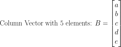
Correlation matrix defines correlation among N variables. It is a symmetric matrix with the element equal to the correlation coefficient between the and the variable. The diagonal elements (correlations of variables with themselves) are always equal to 1.

Sample problem:

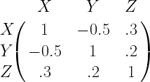
Let’s say we would like to generate three sets of random sequences X,Y,Z with the following correlation relationships.

  1. Correlation co-efficient between X and Y is 0.5
  2. Correlation co-efficient between X and Z is 0.3
  3. Obviously the variable X  correlates with itself 100% – i.e, correlation-coefficient is 1

Putting all these relationships in a compact matrix form, gives the correlation matrix. We take arbitrary correlation value (0.3) for the relationship between Y and Z.

Now, the task is to generate three sets of random numbers X,Y and Z that follows the relationship above. The problem can be addressed in many ways. Two most common methods finding the solution are

  1. Cholesky Decomposition method
  2. Spectral Decomposition ( also called Eigen Vector Decomposition) method

The Cholesky Decomposition method is discussed here.

This article is part of the book
Wireless Communication Systems in Matlab (second edition), ISBN: 979-8648350779 available in ebook (PDF) format and Paperback (hardcopy) format.

Generating Correlated random number using Cholesky Decomposition:

Cholesky decomposition is the matrix equivalent of taking square root operation on a given matrix. As with any scalar values, positive square root is only possible if the given number is a positive (Imaginary roots do exist otherwise). Similarly, if a matrix need to be decomposed into square-root equivalent, the matrix need to be positive definite.

The method discussed here, seeks to decompose the given correlation matrix using Cholesky decomposition.

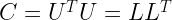
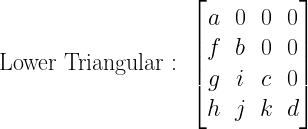
where U and L are upper and lower triangular matrices. We will consider Upper triangular matrix here. Equivalently, lower triangular matrix can also be used, in which case the order of output needs to be reversed.

For this decomposition to work, the correlation matrix should be positive definite. The correlated random sequences (where X,Y,Z are column vectors) that follow the above relationship can be generated by multiplying the uncorrelated random numbers R  with U .

Steps to follow:

Generate three sequences of uncorrelated random numbers R – each drawn from a normal distribution. For this case, the R matrix will be of size where k is the number of  samples we wish to generate and we allocate the k samples in three columns, where the columns indicate the place holder for each variable X, Y and Z. Multiply this matrix with the Cholesky decomposed upper triangular version of the correlation matrix.

Python code

import numpy as np
from scipy.linalg import cholesky
from scipy.stats import pearsonr #to calculate correlation coefficient

#for plotting and visualization
import pandas as pd
import matplotlib.pyplot as plt
%matplotlib inline
plt.style.use('fivethirtyeight')
import seaborn as sns

C = np.array([[1, -0.5, 0.3], 
              [-0.5, 1, 0.2],
              [0.3, 0.2, 1]]) #Construct correlation matrix
U = cholesky(C) #Cholesky decomposition
R = np.random.randn(10000,3) #Three uncorrelated sequences
Rc = R @ U #Array of correlated random sequences

#compute and display correlation coeff from generated sequences
def pearsonCorr(x, y, **kws): 
    (r, _) = pearsonr(x, y) #returns Pearson’s correlation coefficient, 2-tailed p-value)
    ax = plt.gca()
    ax.annotate("r = {:.2f} ".format(r),xy=(.7, .9), xycoords=ax.transAxes)
    
#Visualization
df = pd.DataFrame(data=Rc, columns=['X','Y','Z'])
graph = sns.pairplot(df)
graph.map(pearsonCorr)
Pairplot of correlated random variables generated using Cholesky decomposition (Python)
Figure 1: Pairplot of correlated random variables generated using Cholesky decomposition (Python)

Matlab code

x=[  1  0.5 0.3; 0.5  1  0.3; 0.3 0.3  1 ;]; %Correlation matrix
U=chol(x); %Cholesky decomposition 

R=randn(10000,3); %Random data in three columns each for X,Y and Z
Rc=R*U; %Correlated matrix Rc=[X Y Z]

%Verify Correlation-Coeffs of generated vectors
coeffMatrixXX=corrcoef(Rc(:,1),Rc(:,1));
coeffMatrixXY=corrcoef(Rc(:,1),Rc(:,2));
coeffMatrixXZ=corrcoef(Rc(:,1),Rc(:,3));

%Extract the required correlation coefficients
coeffXX=coeffMatrixXX(1,2) %Correlation Coeff for XX;
coeffXY=coeffMatrixXY(1,2) %Correlation Coeff for XY;
coeffXZ=coeffMatrixXZ(1,2) %Correlation Coeff for XZ;

%Scatterplots
subplot(3,1,1)
plot(Rc(:,1),Rc(:,1),'b.')
title(['Scatterd Plot - X and X calculated \rho=' num2str(coeffXX)])
xlabel('X')
ylabel('X')

subplot(3,1,2)
plot(Rc(:,1),Rc(:,2),'r.')
title(['Scatterd Plot - X and Y calculated \rho=' num2str(coeffXY)])
xlabel('X')
ylabel('Y')

subplot(3,1,3)
plot(Rc(:,1),Rc(:,3),'m.')
title(['Scatterd Plot - X and Z calculated \rho=' num2str(coeffXZ)])
xlabel('X')
ylabel('Z')

Scattered plots to verify the simulated data

Rate this article: Note: There is a rating embedded within this post, please visit this post to rate it.

Further reading

[1] Richard Taylor, “Interpretation of correlation coefficient: A basic review”, Journal of diagnostic medical sonography, Jan/Feb 1990.↗

Topics in this chapter

Random Variables - Simulating Probabilistic Systems
● Introduction
Plotting the estimated PDF
● Univariate random variables
 □ Uniform random variable
 □ Bernoulli random variable
 □ Binomial random variable
 □ Exponential random variable
 □ Poisson process
 □ Gaussian random variable
 □ Chi-squared random variable
 □ Non-central Chi-Squared random variable
 □ Chi distributed random variable
 □ Rayleigh random variable
 □ Ricean random variable
 □ Nakagami-m distributed random variable
Central limit theorem - a demonstration
● Generating correlated random variables
 □ Generating two sequences of correlated random variables
 □ Generating multiple sequences of correlated random variables using Cholesky decomposition
Generating correlated Gaussian sequences
 □ Spectral factorization method
 □ Auto-Regressive (AR) model

Books by the author


Wireless Communication Systems in Matlab
Second Edition(PDF)

Note: There is a rating embedded within this post, please visit this post to rate it.
Checkout Added to cart

Digital Modulations using Python
(PDF ebook)

Note: There is a rating embedded within this post, please visit this post to rate it.
Checkout Added to cart

Digital Modulations using Matlab
(PDF ebook)

Note: There is a rating embedded within this post, please visit this post to rate it.
Checkout Added to cart
Hand-picked Best books on Communication Engineering
Best books on Signal Processing

Solve Triangular Matrix – Forward & Backward Substitution

Key focus: Know the expressions to solve triangular matrix using forward and backward substituting techniques and the FLOPS required for solving it.

Forward Substitution:

Consider a set of equations in a matrix form , where A is a lower triangular matrix with non-zero diagonal elements. The equation is re-written in full matrix form as

It can be solved using the following expressions

From the DSP implementation point of view, computation of requires one FLoating Point Operation per Second (FLOPS) – only one division. Computing will require 3 FLOPS – 1 multiplication, 1 division and 1 subtraction, will require 5 FLOPS – 2 multiplications, 1 division and two subtractions. Thus the computation of will require FLOPS.

Thus the overall FLOPS required for forward substitution is FLOPS

Backward substitution:

Consider a set of equations in a matrix form , where A is a upper triangular matrix with non-zero diagonal elements. The equation is re-written in full matrix form as

Solved using the following algorithm

This one also requires FLOPS.

Rate this article: Note: There is a rating embedded within this post, please visit this post to rate it.

More on Estimation Theory:

[1]An Introduction to Estimation Theory
[2]Bias of an Estimator
[3]Minimum Variance Unbiased Estimators (MVUE)
[4]Maximum Likelihood Estimation
[5]Maximum Likelihood Decoding
[6]Probability and Random Process
[7]Likelihood Function and Maximum Likelihood Estimation (MLE)
[8]Score, Fisher Information and Estimator Sensitivity
[9]Introduction to Cramer Rao Lower Bound (CRLB)
[10]Cramer Rao Lower Bound for Scalar Parameter Estimation
[11]Applying Cramer Rao Lower Bound (CRLB) to find a Minimum Variance Unbiased Estimator (MVUE)
[12]Efficient Estimators and CRLB
[13]Cramer Rao Lower Bound for Phase Estimation
[14]Normalized CRLB - an alternate form of CRLB and its relation to estimator sensitivity
[15]Cramer Rao Lower Bound (CRLB) for Vector Parameter Estimation
[16]The Mean Square Error – Why do we use it for estimation problems
[17]How to estimate unknown parameters using Ordinary Least Squares (OLS)
[18]Essential Preliminary Matrix Algebra for Signal Processing
[19]Why Cholesky Decomposition ? A sample case:
[20]Tests for Positive Definiteness of a Matrix
[21]Solving a Triangular Matrix using Forward & Backward Substitution
[22]Cholesky Factorization - Matlab and Python
[23]LTI system models for random signals – AR, MA and ARMA models
[24]Comparing AR and ARMA model - minimization of squared error
[25]Yule Walker Estimation
[26]AutoCorrelation (Correlogram) and persistence – Time series analysis
[27]Linear Models - Least Squares Estimator (LSE)
[28]Best Linear Unbiased Estimator (BLUE)

Books by the author


Wireless Communication Systems in Matlab
Second Edition(PDF)

Note: There is a rating embedded within this post, please visit this post to rate it.
Checkout Added to cart

Digital Modulations using Python
(PDF ebook)

Note: There is a rating embedded within this post, please visit this post to rate it.
Checkout Added to cart

Digital Modulations using Matlab
(PDF ebook)

Note: There is a rating embedded within this post, please visit this post to rate it.
Checkout Added to cart
Hand-picked Best books on Communication Engineering
Best books on Signal Processing

Matrix Algebra for Signal Processing

Key focus : Essential matrix algebra: formation of matrices, determinants, rank, inverse & transpose of matrix and solving simultaneous equations.

I thought of making a post on Cholesky Decomposition, which is a very essential technique in digital signal processing applications like generating correlated random variables, solving linear equations, channel estimation etc.., But jumping straight to the topic of Cholesky Decomposition will leave many flummoxed/confused. So I decided to touch on some essentials in basic matrix algebra before taking up advanced topics.

Prerequisite:

Basic knowledge on topics like formation of matrices, determinants, rank of a matrix, inverse & transpose of matrix, solving a system of simultaneous equation using matrix algebra.

The prerequisites listed above being fulfilled, you will learn different types of matrices in this post.

1. Vector

A matrix with only one row or one column.

2. Transpose of a Matrix

Transpose of a matrix is formed by interchanging the elements from row to columns. For example, the first row of the matrix becomes first column in the transpose matrix, second row of the matrix becomes second column in the transpose matrix and so on.

3. Square Matrix:

Matrix with equal number of rows and columns.
(Note: The sample matrices shown below are of 3×3 dimension. They can be readily extended to nxn dimension)

Square Matrix is further classified into

4. Symmetric Matrix :

If a square matrix and its transpose are equal, then it is called a symmetric square matrix or simply symmetric matrix.

5. Diagonal Matrix

A special kind of symmetric matrix, with zeros in off-diagonal locations.

6. Scalar matrix

A special kind of diagonal matrix, with the equal values at the diagonal

7. Identity Matrix

It is a special type of scalar matrix, where the leading diagonals are one. It is denoted by I

8. Inverse of a Matrix or the notion of non-Singular Matrix:

Inverse matrices are defined for square matrices. For non-square matrices, inverses do not exist. The product of a square matrix and its inverse yields an identity matrix.
For a square matrix A.

Here denotes the inverse of square matrix .

It is possible to have a square matrix but not invertible. Such non-invertible square matrices are called
Singular Matrices. Matrix that are invertible are called non-singular matrices.

9. Singular Matrix:

A non-invertible square matrix. Inverse does not exist.

10. Orthogonal Matrix

An invertible square matrix, whose transpose and inverse are equal. If for an invertible square matrix A,

then, the matrix or equivalently is called an orthogonal matrix.

11. Complex Matrix :

A matrix with complex elements.

12. Complex Square Matrix

A complex matrix with with equal number of rows and columns

13. Conjugate Transpose or Hermitian Transpose:

Similar to the transpose of a matrix defined above. But the only difference is : put the complex conjugate form of the element when interchanging from rows to columns. For a complex square matrix , the conjugate transpose is denoted by

14. Hermitian Matrix:

A complex square matrix whose conjugate transpose is equal to its own. For a complex square matrix , the Hermitian Matix is denoted by . For a Hermitian matrix, the element of the complex square matrix located at i-th row and j-th column will be equal to the complex conjugate of the element located at j-th row and i-th column.

That is,

15. Triangular Matrix:

A special type of square matrix. Further classified into : lower triangular and upper triangular matrix. For a lower triangular matrix, all the elements above the main diagonal are zeros.For an upper triangular matrix, all the elements below the main diagonal are zeros.

16. Positive-Definite Matrix:

It is defined for both real matrices and complex matrices. It is matrix equivalent to positivity of real numbers. For example, the numbers +3,+5 and +6 are definitely positive. Similarly a positive definite matrix is defined to be definitely positive if it satisfies the following condition.

For real case: A n x n symmetric square real matrix – is said to be positive definite for all if and only if,

For complex case: A n x n symmetric square complex matrix – is said to be positive definite for all if and only if,

17. Positive-semi-definite Matrix:

It is defined for both real matrices and complex matrices. It is matrix equivalent to semi-positivity of real numbers. For example, the numbers +3,+5 and +6 are definitely positive. But the set is not positive definite since it includes a zero element which is neither positive nor negative. Similarly a positive semi-definite matrix is defined to be semi-definitely positive if it satisfies the following condition.

For real case: A n x n symmetric square real matrix – is said to be positive semi-definite for all if and only if,

For complex case: A n x n symmetric square complex matrix – is said to be positive semi-definite for all if and only if,

Note : The notation stands for a set of real numbers. The notation denotes a set of n real numbers in n-dimensional space.

18. Negative-Definite Matrix:

It is defined for both real matrices and complex matrices. It is matrix equivalent to negativity of real numbers. For example, the numbers -3,-5 and -6 are definitely negative. Similarly a negative definite matrix is defined to be definitely negative if it satisfies the following condition.

For real case: A n x n symmetric square real matrix – is said to be negative definite for all if and only if,

For complex case: A n x n symmetric square complex matrix – is said to be negative definite for all if and only if,

Note : The notation stands for a set of real numbers. The notation denotes a set of n real numbers in n-dimensional space.

19. Negative-semi-definite Matrix:

It is defined for both real matrices and complex matrices. It is matrix equivalent to semi-negativity of real numbers. For example, the numbers -3,-5 and -6 are definitely negative. But the set is not negative definite since it includes a zero element which is neither positive nor negative. Similarly a negative semi-definite matrix is defined to be semi-definitely negative if it satisfies the following condition.

For real case: A n x n symmetric square real matrix – is said to be negative semi-definite for all if and only if,

For complex case: A n x n symmetric square complex matrix – is said to be negative semi-definite for all if and only if,

Note : The notation stands for a set of real numbers. The notation denotes a set of n real numbers in n-dimensional space.

20. Indefinite Matrix :

A Matrix, that is neither positive definite, positive semi-definite, negative definite nor negative semi-definite is called an indefinite Matrix.

Rate this article: Note: There is a rating embedded within this post, please visit this post to rate it.

External References:

[1] Vector
[2] Transpose of a Matrix
[3] Square Matrix
[4] Symmetric Matrix
[5] Diagonal Matrix
[6] Scalar Matrix
[7] Identity Matrix
[8] Inverse Matrix
[9] Singular Matrix
[10] Orthogonal Matrix
[11] Complex Matrix
[12] Complex Square Matrix
[13] Conjugate Transpose
[14] Hermitian Matrix
[15] Triangular Matirx
[16] Positive definite, negative definite and semi-definite Matrices