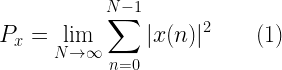
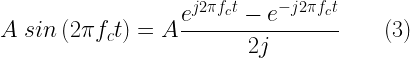
Let x(t) be a sine wave of amplitude A and frequency fc represented by the following equation.
When represented in frequency domain, it will look like the one on the right side plot in the following figure. This is evident from the fact that the sinewave can be mathematically represented by applying Euler’s formula.
Taking the Fourier transform of x(t) to represent it in frequency domain,
When considering the amplitude part,the above decomposition gives two spikes of amplitude A/2 on either side of the frequency domain at fc and -fc.
Figure 1: Time domain representation and frequency spectrum of a pure sinewave
Squaring the amplitudes gives the magnitude of power of the individual spikes/frequency components. The power spectrum is plotted below.
Figure 2: Power spectrum of a pure sinewave
Thus if the pure sinewave is of amplitude A=1V and frequency=100Hz, the power spectrum will have two spikes of value at 100 Hz and -100 Hz frequencies. The total power will be
Let’s verify this through simulation.
Simulation and Verification
A sine wave of 100 Hz frequency and amplitude 1V is taken for the experiment.
A=1; %Amplitude of sine wave
Fc=100; %Frequency of sine wave
Fs=1000; %Sampling rate - oversampled by the rate of 10
Ts=1/Fs; %Sampling period
nCycles=200; %Number of cycles of the sinewave

subplot(2,1,1);
t=0:Ts:nCycles/Fc-Ts; %Time base
x=A*sin(2*pi*Fc*t); %Sinusoidal function
stem(t,x); %Plot command
A sinusoidal wave of 10 cycles is plotted here
Figure 3: Sine wave generated in Matlab
Matlab’s Norm function:
Matlab’s basic installation comes with “norm” function. The p-norm in Matlab is computed as
By default, the single argument norm function computed 2-norm given as
To compute the total power of the signal x[n] (as in equation (1) above), all we have to do is – compute norm(x), square it and divide by the length of the signal.
L=length(x);
P=(norm(x)^2)/L;
sprintf('Power of the Signal from Time domain %f',P);
The above given piece of code will result in the following output
Power of the Signal from Time domain 0.500000
Verifying the total Power by DFT : Frequency Domain
Here, the total power is verified by applying DFT on the sinusoidal sequence. The sinusoidal sequence x[n] is represented in frequency domain X[f] using Matlab’s FFT function. The power associated with each frequency point is computed as
Finally, the total power is calculated as the sum of all the points in the frequency domain representation.
X = fft(x);
Px=sum(X.*conj(X))/(L^2); %Compute power with proper scaling.
subplot(2,1,2)
% Plot single-sided amplitude spectrum.
stem(Px);
sprintf('Total Power of the Signal from DFT %f',P);
Result:
Total Power of the Signal from DFT 0.500000
Figure 4: Power spectrum of a pure sinewave simulated in Matlab
A word on Matlab’s FFT: Matlab’s FFT is optimized for faster performance if the transform length is a power of 2. The following snippet of code simply calls “fft” without the transform length. In this case, the window length and the transform length are the same. This is to simplify the calculation of power. You can re-write the call to the FFT routine with transform length set to next power of two which is greater than or equal to the window length (sequence length). Then the step to compute total power will be differing slightly in the denominator. But that will not improve resolution (Remember : zero padding to compute FFT will not improve resolution).
Also note that in the above simulation we are using a pure sinusoid. The entire sequence of sinusoid defined all the cycles completely. There are no discontinuities in the sequence. If you call FFT with the transform length set to next power of 2 (as given in Matlab manuals), it will pad additional zeros to the sequence and creates discontinuities in the FFT computation. This will lead to spectral leakage. FFT and spectral leakage is discussed here.
Rate this article: Note: There is a rating embedded within this post, please visit this post to rate it.
Key focus: Clearly understand the terms: power and energy of a signal, their mathematical definition, physical significance and computation in signal processing context.
Energy of a signal:
Defining the term “size”:
In signal processing, a signal is viewed as a function of time. The term “size of a signal” is used to represent “strength of the signal”. It is crucial to know the “size” of a signal used in a certain application. For example, we may be interested to know the amount of electricity needed to power a LCD monitor as opposed to a CRT monitor. Both of these applications are different and have different tolerances. Thus the amount of electricity driving these devices will also be different.
A given signal’s size can be measured in many ways. Given a mathematical function (or a signal equivalently), it seems that the area under the curve, described by the mathematical function, is a good measure of describing the size of a signal. A signal can have both positive and negative values. This may render areas that are negative. Due to this effect, it is possible that the computed values cancel each other totally or partially, rendering incorrect result. Thus the metric function of “area under the curve” is not suitable for defining the “size” of a signal. Now, we are left with two options : either 1) computation of the area under the absolute value of the function or 2) computation of the area under the square of the function. The second choice is favored due to its mathematical tractability and its similarity to Euclidean Norm which is used in signal detection techniques (Note: Euclidean norm – otherwise called L2 norm or 2-norm[1] – is often considered in signal detection techniques – on the assumption that it provides a reasonable measure of distance between two points on signal space. It is computed as Euclidean distance in detection theory).
Going by the second choice of viewing the “size” as the computation of the area under the square of the function, the energy of a continuous-time complex signal \(x(t)\) is defined as
\[E_x = \int_{-\infty}^{\infty} |x(t)|^2 dt\]
If the signal \(x(t)\) is real, the modulus operator in the above equation does not matter.
This is called “Energy” in signal processing terms. This is also a measure of signal strength. This definition can be applied to any signal (or a vector) irrespective of whether it possesses actual energy (a basic quantitative property as described by physics) or not. If the signal is associated with some physical energy, then the above definition gives the energy content in the signal. If the signal is an electrical signal, then the above definition gives the total energy of the signal (in Joules) dissipated over a 1 Ohm resistor.
Actual Energy – physical quantity:
To know the actual energy of the signal \(E\), one has to know the value of load \(Z\) the signal is driving and also the nature the electrical signal (voltage or current). For a voltage signal, the above equation has to be scaled by a factor of \(1/Z\).
\[E = ZE_x = Z \int_{-\infty}^{\infty} |x(t)|^2 dt\]
Here, \(Z\) is the impedance driven by the signal \(x(t)\) , \(E_x\) is the signal energy (signal processing term) and \(E\) is the Energy of the signal (physical quantity) driving the load \( Z\)
Energy in discrete domain:
In the discrete domain, the energy of the signal is given by
The energy is finite only if the above sum converges to a finite value. This implies that the signal is “squarely-summable“. Such a signal is called finite energy signal.
What if the given signal does not decay with respect to time (as in a continuous sine wave repeating its cycle infinitely) ? The energy will be infinite and such a signal is “not squarely-summable” in other words. We need another measurable quantity to circumvent this problem.This leads us to the notion of “Power”
Power:
Power is defined as the amount of energy consumed per unit time. This quantity is useful if the energy of the signal goes to infinity or the signal is “not-squarely-summable”. For “non-squarely-summable” signals, the power calculated by taking the snapshot of the signal over a specific interval of time as follows
1) Take a snapshot of the signal over some finite time duration 2) Compute the energy of the signal \(E_x\) 3) Divide the energy by number of samples taken for computation \(N\) 4) Extend the limit of number of samples to infinity \(N\rightarrow \infty \). This gives the total power of the signal.
In discrete domain, the total power of the signal is given by
Following equations are different forms of the same computation found in many text books. The only difference is the number of samples taken for computation. The denominator changes according to the number of samples taken for computation.
A signal can be classified based on its power or energy content. Signals having finite energy are energy signals. Power signals have finite and non-zero power.
Energy Signal :
A finite energy signal will have zero TOTAL power. Let’s investigate this statement in detail. When the energy is finite, the total power will be zero. Check out the denominator in the equation for calculating the total power. When the limit \(N\rightarrow \infty\), the energy dilutes to zero over the infinite duration and hence the total power becomes zero.
Power Signal:
Signals whose total power is finite and non-zero. The energy of the power signal will be infinite. Example: Periodic sequences like sinusoid. A sinusoidal signal has finite, non-zero power but infinite energy.
A signal cannot be both an energy signal and a power signal.
Neither an Energy signal nor a Power signal:
Signals can also be a cat on the wall – neither an energy signal nor a power signal. Consider a signal of increasing amplitude defined by,
\[x(n) = n\]
For such a signal, both the energy and power will be infinite. Thus, it cannot be classified either as an energy signal or as a power signal.
A random process (or signal for your visualization) with a constant power spectral density (PSD) function is a white noise process.
Power Spectral Density
Power Spectral Density function (PSD) shows how much power is contained in each of the spectral component. For example, for a sine wave of fixed frequency, the PSD plot will contain only one spectral component present at the given frequency. PSD is an even function and so the frequency components will be mirrored across the Y-axis when plotted. Thus for a sine wave of fixed frequency, the double sided plot of PSD will have two components – one at +ve frequency and another at –ve frequency of the sine wave. (Know how to plot PSD/FFT in Python & in Matlab)
Gaussian and Uniform White Noise:
A white noise signal (process) is constituted by a set of independent and identically distributed (i.i.d) random variables. In discrete sense, the white noise signal constitutes a series of samples that are independent and generated from the same probability distribution. For example, you can generate a white noise signal using a random number generator in which all the samples follow a given Gaussian distribution. This is called White Gaussian Noise (WGN) or Gaussian White Noise. Similarly, a white noise signal generated from a Uniform distribution is called Uniform White Noise.
Gaussian Noise and Uniform Noise are frequently used in system modelling. In modelling/simulation, white noise can be generated using an appropriate random generator. White Gaussian Noise can be generated using randn function in Matlab which generates random numbers that follow a Gaussian distribution. Similarly, rand function can be used to generate Uniform White Noise in Matlab that follows a uniform distribution. When the random number generators are used, it generates a series of random numbers from the given distribution. Let’s take the example of generating a White Gaussian Noise of length 10 using randn function in Matlab – with zero mean and standard deviation=1.
This simply generates 10 random numbers from the standard normal distribution. As we know that a white process is seen as a random process composing several random variables following the same Probability Distribution Function (PDF). The 10 random numbers above are generated from the same PDF (standard normal distribution). This condition is called “identically distributed” condition. The individual samples given above are “independent” of each other. Furthermore, each sample can be viewed as a realization of one random variable. In effect, we have generated a random process that is composed of realizations of 10 random variables. Thus, the process above is constituted from “independent identically distributed” (i.i.d) random variables.
Strictly and weakly defined white noise:
Since the white noise process is constructed from i.i.d random variable/samples, all the samples follow the same underlying probability distribution function (PDF). Thus, the Joint Probability Distribution function of the process will not change with any shift in time. This is called a stationary process. Hence, this noise is a stationary process. As with a stationary process which can be classified as Strict Sense Stationary (SSS) and Wide Sense Stationary (WSS) processes, we can have white noise that is SSS and white noise that is WSS. Correspondingly they can be called strictly defined white noise signal and weakly defined white noise signal.
What’s with Covariance Function/Matrix ?
A white noise signal, denoted by \(x(t)\), is defined in weak sense is a more practical condition. Here, the samples are statistically uncorrelated and identically distributed with some variance equal to \(\sigma^2\). This condition is specified by using a covariance function as
\[COV \left(x_i, x_j \right) = \begin{cases} \sigma^2, & \quad i = j \\ 0, & \quad i \neq j \end{cases}\]
Why do we need a covariance function? Because, we are dealing with a random process that is composed of \(n\) random variables (10 variables in the modelling example above). Such a process is viewed as multivariate random vector or multivariate random variable.
For multivariate random variables, Covariance function specified how each of the \(n\) variables in the given random process behaves with respect to each other. Covariance function generalizes the notion of variance to multiple dimensions.
The above equation when represented in the matrix form gives the covariance matrix of the white noise random process. Since the random variables in this process are statistically uncorrelated, the covariance function contains values only along the diagonal.
The matrix above indicates that only the auto-correlation function exists for each random variable. The cross-correlation values are zero (samples/variables are statistically uncorrelated with respect to each other). The diagonal elements are equal to the variance and all other elements in the matrix are zero.The ensemble auto-correlation function of the weakly defined white noise is given by This indicates that the auto-correlation function of weakly defined white noise process is zero everywhere except at lag \(\tau=0\).
\[R_{xx}(\tau) = E \left[ x(t) x^*(t-\tau)\right] = \sigma^2 \delta (\tau)\]
Wiener-Khintchine Theorem states that for Wide Sense Stationary Process (WSS), the power spectral density function \(S_{xx}(f)\) of a random process can be obtained by Fourier Transform of auto-correlation function of the random process. In continuous time domain, this is represented as
\[S_{xx}(f) = F \left[R_{xx}(\tau) \right] = \int_{-\infty}^{\infty} R_{xx} (\tau) e ^{- j 2 \pi f \tau} d \tau\]
For the weakly defined white noise process, we find that the mean is a constant and its covariance does not vary with respect to time. This is a sufficient condition for a WSS process. Thus we can apply Weiner-Khintchine Theorem. Therefore, the power spectral density of the weakly defined white noise process is constant (flat) across the entire frequency spectrum (Figure 1). The value of the constant is equal to the variance or power of the noise signal.
\[S_{xx}(f) = F \left[R_{xx}(\tau) \right] = \int_{-\infty}^{\infty} \sigma^2 \delta (\tau) e ^{- j 2 \pi f \tau} d \tau = \sigma^2 \int_{-\infty}^{\infty} \delta (\tau) e ^{- j 2 \pi f \tau} = \sigma^2\]
Figure 1: Weiner-Khintchine theorem illustrated
Testing the characteristics of White Gaussian Noise in Matlab:
Generate a Gaussian white noise signal of length \(L=100,000\) using the randn function in Matlab and plot it. Let’s assume that the pdf is a Gaussian pdf with mean \(\mu=0\) and standard deviation \(\sigma=2\). Thus the variance of the Gaussian pdf is \(\sigma^2=4\). The theoretical PDF of Gaussian random variable is given by
subplot(2,1,2)
n=100; %number of Histrogram bins
[f,x]=hist(X,n);
bar(x,f/trapz(x,f)); hold on;
%Theoretical PDF of Gaussian Random Variable
g=(1/(sqrt(2*pi)*sigma))*exp(-((x-mu).^2)/(2*sigma^2));
plot(x,g);hold off; grid on;
title('Theoretical PDF and Simulated Histogram of White Gaussian Noise');
legend('Histogram','Theoretical PDF');
xlabel('Bins');
ylabel('PDF f_x(x)');
Figure 3: Plot of simulated & theoretical PDF for Gaussian RV
Compute the auto-correlation function of the white noise. The computed auto-correlation function has to be scaled properly. If the ‘xcorr’ function (inbuilt in Matlab) is used for computing the auto-correlation function, use the ‘biased’ argument in the function to scale it properly.
figure();
Rxx=1/L*conv(flipud(X),X);
lags=(-L+1):1:(L-1);

%Alternative method
%[Rxx,lags] =xcorr(X,'biased');
%The argument 'biased' is used for proper scaling by 1/L
%Normalize auto-correlation with sample length for proper scaling

plot(lags,Rxx);
title('Auto-correlation Function of white noise');
xlabel('Lags')
ylabel('Correlation')
grid on;
Figure 4: Autocorrelation function of generated noise
Simulating the PSD:
Simulating the Power Spectral Density (PSD) of the white noise is a little tricky business. There are two issues here 1) The generated samples are of finite length. This is synonymous to applying truncating an infinite series of random samples. This implies that the lags are defined over a fixed range. ( FFT and spectral leakage – an additional resource on this topic can be found here) 2) The random number generators used in simulations are pseudo-random generators. Due these two reasons, you will not get a flat spectrum of psd when you apply Fourier Transform over the generated auto-correlation values.The wavering effect of the psd can be minimized by generating sufficiently long random signal and averaging the psd over several realizations of the random signal.
Simulating Gaussian White Noise as a Multivariate Gaussian Random Vector:
To verify the power spectral density of the white noise, we will use the approach of envisaging the noise as a composite of \(N\) Gaussian random variables. We want to average the PSD over \(L\) such realizations. Since there are \(N\) Gaussian random variables (\(N\) individual samples) per realization, the covariance matrix \( C_{xx}\) will be of dimension \(N \times N\). The vector of mean for this multivariate case will be of dimension \(1 \times N\).
Cholesky decomposition of covariance matrix gives the equivalent standard deviation for the multivariate case. Cholesky decomposition can be viewed as square root operation. Matlab’s randn function is used here to generate the multi-dimensional Gaussian random process with the given mean matrix and covariance matrix.
%Verifying the constant PSD of White Gaussian Noise Process
%with arbitrary mean and standard deviation sigma

mu=0; %Mean of each realization of Noise Process
sigma=2; %Sigma of each realization of Noise Process

L = 1000; %Number of Random Signal realizations to average
N = 1024; %Sample length for each realization set as power of 2 for FFT

%Generating the Random Process - White Gaussian Noise process
MU=mu*ones(1,N); %Vector of mean for all realizations
Cxx=(sigma^2)*diag(ones(N,1)); %Covariance Matrix for the Random Process
R = chol(Cxx); %Cholesky of Covariance Matrix
%Generating a Multivariate Gaussian Distribution with given mean vector and
%Covariance Matrix Cxx
z = repmat(MU,L,1) + randn(L,N)*R;
Compute PSD of the above generated multi-dimensional process and average it to get a smooth plot.
%By default, FFT is done across each column - Normal command fft(z)
%Finding the FFT of the Multivariate Distribution across each row
%Command - fft(z,[],2)
Z = 1/sqrt(N)*fft(z,[],2); %Scaling by sqrt(N);
Pzavg = mean(Z.*conj(Z));%Computing the mean power from fft

normFreq=[-N/2:N/2-1]/N;
Pzavg=fftshift(Pzavg); %Shift zero-frequency component to center of spectrum
plot(normFreq,10*log10(Pzavg),'r');
axis([-0.5 0.5 0 10]); grid on;
ylabel('Power Spectral Density (dB/Hz)');
xlabel('Normalized Frequency');
title('Power spectral density of white noise');
Figure 5: Power spectral density of generated noise
The PSD plot of the generated noise shows almost fixed power in all the frequencies. In other words, for a white noise signal, the PSD is constant (flat) across all the frequencies (\(- \infty\) to \(+\infty\)). The y-axis in the above plot is expressed in dB/Hz unit. We can see from the plot that the \(constant \; power = 10 log_{10}(\sigma^2) = 10 log_{10}(4) = 6\; dB\).
Application
In channel modeling, we often come across additive white Gaussian noise (AWGN) channel. To know more about the channel model and its simulation, continue reading this article: Simulate AWGN channel in Matlab & Python.
Rate this article: Note: There is a rating embedded within this post, please visit this post to rate it.
Note: There is a rating embedded within this post, please visit this post to rate it.
Researchers, working on Ultra-Parallel Visible Light Communications (UP-VLC) project, have demonstrated 3.5Gpbs free space data transmission via three separate micro-LEDs that emit red, blue and green colours. In effect, combining the three colours (that makes up for white colour), researchers say that achieving data rates over 10Gbps is feasible.
The technology enabler here is called – “Li-Fi”, a term coined by Prof. Harold Haas of University of Edinburgh, uses LED lights as medium of data transmission. Li-Fi, academically referred as “Visible Light Communication”, aims to use existing micro- LED light bulbs for both illumination and communication.
With the advent of this technology, soon you will see all the illuminated spots in offices, houses or any other place turning into internet hotspots streaming high quality data. It has become a hot topic and soon many big corporations will jump on to the Li-Fi bandwagon.
It all started with Prof. Hass’s research group demonstrating the proof-of-concept results that exploited the higher peak-to-average ratio (PAR) property of Orthogonal Frequency Division Multiplexing (OFDM) systems. PAR, otherwise called “Crest Factor”, is a disadvantage in RF communications. The research group have used this property to turn commercially available LED bulbs to ultra-high speed wireless hotspots. Later, this work was featured in TIME magazine’s “50 Best inventions of the year 2011” and Nobel Laureate Prof. Hänsch listed this work in his book titled “100 ground-breaking ideas” that could shape the next century.
Using OFDM, micro-LED light bulbs are enabled to handing millions of light-intensity-changes per second. Essentially, the micro-LED bulbs are switched on and off depending on the input bits –‘0’ or ‘1’. The switching is done at such a high speed that it is undetectable by human eye. Thus both un-flickering-illumination and high-speed-communication are achievable under this condition.
Li-Fi carries the promise of breaking the bandwidth-crunch suffered by existing wireless systems. The demand for more bandwidth is skyrocketing day by day with the proliferation of wireless enabled devices. The crunch faced by Radio-Frequency (RF) systems, is also compounded by complex government regulations, needs of a growing base of customers and risking of the performance issues due to these challenges.
Li-Fi is essentially a wireless system. It uses the visible light region of the electromagnetic spectrum which is 10,000 times larger than the microwave region of the electromagnetic spectrum. This opens up the utilizable frequencies to the order of terahertz level. It will not interfere with existing devices and it can be used in areas where there is extensive RF noise or in places where RF frequencies are restricted (like in airplanes).
Watch the TED talk – “Wireless data from every light bulb”- where Prof Haas demonstrates the capability of Li-Fi technology system prototype (using a desk-lamp) that steams a HD movie in real-time.
The goal of timing recovery is to estimate and correct the sampling instants and phase at the receiver, such that it allows the receiver to decode the transmitted symbols reliably.
What is Symbol timing Recovery :
When transmitting data across a communication system, three things are important: frequency of transmission, phase information and the symbol rate.
In coherent detection/demodulation, both the transmitter and receiver posses the knowledge of exact symbol sampling timing and symbol phase (and/or symbol frequency). While everything is set at the transmitter, the receiver is at the mercy of recovery algorithms to regenerate these information from the incoming signal itself. If the transmission is a passband transmission, the carrier recovery algorithm also recovers the carrier frequency. For phase sensitive systems like BPSK, QPSK etc.., the carrier recovery algorithm recovers the symbol phase so that it is synchronous with the transmitted symbol.
The first part in such a receiver architecture of a MPSK transmitting system is multiplying the incoming signal with sine and cosine components of the carrier wave.
The sine and cosine components are generated using a carrier recovery block (Phase Lock Loop (PLL) or setting a local oscillator to track the variations).
Once the in-phase and quadrature signals are separated out properly, the next task is to match each symbol with the transmitted pulse shape such that the overall SNR of the system improves.
Implementing this in digital domain, the architecture described so far would look like this (Note: the subscript of the incoming signal has changed from analog domain to digital domain – i.e. to )
In the digital architecture above, the matched filter is implemented as a simple finite impulse response (FIR) filter whose impulse response is matched to that of the transmitter pulse shape. It helps the receiver in timing recovery and also it improves the overall SNR of the system by suppressing some amount of noise. The incoming signal up to the point before the matched filter, may have fluctuations in the amplitude. The matched filter also behaves like an averaging filter that smooths out the variations in the signal.
Note that in this digital version, the incoming signal is already a sampled signal. It has already passed through an analog to digital converter that sampled the signal at some sampling rate. From the symbol perspective, the symbols have to be sampled at optimum sampling instant to extract its content properly.
This requires a re-sampler, which resamples the averaged signal at the optimum sampling instant. If the original sampling instant is before or after the optimum sampling point, the timing recovery signal will help to re-sample (re-adjust sampling times) accordingly.
An alternate data pattern (symbols) – [+1,-1,+1,+1,\cdots,] is transmitted across the channel. Assume that each symbol occupies Tsym=8 sample time.
clear all; clc;
n=10; %Number of data symbols
Tsym=8; %Symbol time interms of sample time or oversampling rate equivalently
%data=2*(rand(n,1)<0.5)-1;
data=[1 -1 1 -1 1 -1 1 -1 1 -1]'; %BPSK data
bpsk=reshape(repmat(data,1,Tsym)',n*Tsym,1); %BPSK signal

figure('Color',[1 1 1]);
subplot(3,1,1);
plot(bpsk);
title('Ideal BPSK symbols');
xlabel('Sample index [n]');
ylabel('Amplitude')
set(gca,'XTick',0:8:80);
axis([1 80 -2 2]); grid on;
Lets add white gaussian noise (awgn). A random noise of standard deviation 0.25 is generated and added with the generated BPSK symbols.
noise=0.25*randn(size(bpsk)); %Adding some amount of noise
received=bpsk+noise; %Received signal with noise

subplot(3,1,2);
plot(received);
title('Transmitted BPSK symbols (with noise)');
xlabel('Sample index [n]');
ylabel('Amplitude')
set(gca,'XTick',0:8:80);
axis([1 80 -2 2]); grid on;
From the first plot, we see that the transmitted pulse is a rectangular pulse that spans Tsym samples. In the illustration, Tsym=8. The best averaging filter (matched filter) for this case is a rectangular filter (though they are not preferred in practice, I am just using it for simplifying the illustration) that spans 8 samples. Such a rectangular pulse can be mathematically represented in terms of unit step function as
The resulting rectangular pulse will have a value of 0.5 at the edges of the sampling instants (index 0 and 7) and a value of ‘1’ at the remaining indices in between the edges. Such a rectangular function is indicated below.
The incoming signal is convolved with the averaging filter and the resultant output is given below
We can note that the averaged output peaks at the locations where the symbol transition occurs. Thus, when the signal is sampled at those ideal locations, the BPSK symbols [+1,-1,+1, …] can be recovered perfectly.
But the problem here is: “How does the receiver know the ideal sampling instants?”. The solution is “someone has to supply those ideal sampling instants”. A symbol time recovery circuit is used for this purpose.
Coming back to the receiver architecture, lets add a symbol time recovery circuit that supplies the recovered timing instants. The signal will be re-sampled at those instants supplied by the recovery circuit.
The Algorithm behind Symbol Timing Recovery:
Different algorithms exist for symbol timing recovery and synchronization. An “Early/Late Symbol Recovery algorithm” is illustrated here.
The algorithm starts by selecting an arbitrary sample at some time (denoted by T). It captures the two adjacent samples (on either side of the sampling instant T) that are separated by δ seconds. The sample at the index T-δ is called Early Sample and the sample at the index T+δ is called Late Sample. The timing error is generated by comparing the amplitudes of the early and late samples. The next symbol sampling time instant is either advanced or delayed based on the sign of difference between the early and late sample.
1) If the Early Sample = Late Sample : The peak occurs at the on-time sampling instant T. No adjustment in the timing is needed. 2) If |Early Sample| > |Late Sample| : Late timing, the sampling time is offset so that the next symbol is sampled T-δ/2 seconds after the current sampling time. 3) If |Early Sample| < |Late Sample| : Early timing, the sampling time is offset so that the next symbol is sampled T+δ/2 seconds after the current sampling time.
These three situations are shown next.
There exist many variations to the above mentioned algorithm. The Early/Late synchronization technique given here is the simplest one taken for illustration.
Let’s complete the architecture with a signal quantization and constellation de-mapping block which gives out the estimated demodulated symbols.
Rate this article: Note: There is a rating embedded within this post, please visit this post to rate it.
Note: There is a rating embedded within this post, please visit this post to rate it.
What is Probability?
Probability is a branch of mathematics that deals with uncertainty. The term “probability” is used to quantify the degree of belief or confidence that something is true (or false). It gives us the likelihood of occurrence of a given event. It is expressed as a number that could take any value in the closed interval [0,1]
Consider the following experiment describing a simple communication system. A user transmits data through a noisy medium and another user receives it. Here, the sender utters a single alphabet on the phone. Due to the noise characteristics of the communication medium, we do not know whether the user at the destination will be able to hear what the sender has already spoken. Before performing the experiment, we would like to know the likelihood that the user at the destination hears the particular syllable (given the noise characteristics). This likelihood of the particular event is called probability of the event.
Experiment:
Any activity that can produce observable results is called an experiment. For example, tossing a coin (observable results: Head/Tail), Rolling a die (observable results: numbers on the faces of the die), drawing a card from a deck (observable results: symbols, numbers and alphabets on the cards), sending & receiving bits in a communication system (observable results: bits/alphabets transferred or voltage level at the receiver).
Sample Space:
Given an experiment, the sample space comprises a set of all possible outcomes of the experiment. It plays the role of the universal set when modeling the experiment. It is denoted by the letter – ‘S’. Following examples illustrate the sample spaces for various experiments.
Event:
It is also a set of outcomes of an experiment. It is a subset of sample space. Each time the experiment is run, either a particular event occurs or it does not occur. Events are associated with a probability number.
Types of Events:
Events can be classified according to their relationship with one another. The following table shows the classification of events and their definition.
Computing Probability:
The proability of the occurrence of an event (say ‘A’) is given by the ratio of number of ways that particular event can happen and the total number of all possible outcomes.
For example, consider the experiment of an unbiased rolling of a die. The sample space is given by S={1,2,3,4,5,6}. Let’s say that an event is defined as getting ‘4’ when you roll the die. The probability of getting the face with ‘4’ (event) can be calculated as follows.
Axioms of Probability:
Following definitions are assumed for the axioms listed below: ‘S’ denotes the sample space of an experiment, ‘A’ and ‘B’ are events and P(A) denotes the probability of occurrence of event ‘A’.
Properties of Probability:
The definition of probability – has some properties as listed below.
Here the symbol Ø indicates null event, Ā indicates that the event A is NOT occuring.
Joint probability and Marginal probability:
Joint probability is defined as the probability that two or more events occur simultaneously. For two events A and B, the joint probability is denoted by P(A,B) or P(A∩B).
Given two or more events, the marginal probability is the probability of occurrence of a single event. It is also called a-priori probability.
The following table illustrates the concept of computing the joint and marginal probabilities. Here, four events (P, Q, R, S) are used for illustration. For example, the table indicates that the probability of occurrence of both events R & Q is given by b/n. This is the joint probability of R and Q. Adding all the probabilities either row wise or column wise gives us the marginal probability of a single event. For example, adding a/n and b/n gives the marginal probability of event similarly, adding a/n and c/n gives the marginal probability of event P.
Conditional probability or Posteriori probability:
Conditional probabilities (also called posteriori probability) deal with dependent events. It is used to calculate the probability of an event given that some other event has already occurred.
It is denoted as P(B|A)–meaning that ‘the probability of event B given that the event A has occurred already’. It is called “a-posteriori” because it is only available “after” observing A (the first event).
The conditional probability P(B|A) is mathematically computed as
Note: There is a rating embedded within this post, please visit this post to rate it.
When simulating digital modulations in Matlab, it is useful to verify the simulated BER performance curves against theoretical BER curves.Matlab has an inbuilt visualization tool, ‘BERTOOL’, for this purpose.
Matlab’s BERTOOL supports 6 types of digital modulations over 3 types of channel for plotting theoretical BER. The six supported modulations are PSK,DPSK,OQPSK,PAM,QAM,FSK and the three channel types are : AWGN,Rayleigh,Rician. It also has options to set diversity order, channel coding, synchronization method and demodulation type(coherent/non-coherent).
A brief intro to the tool is given here. You might need to install communication toolbox for invoking this tool.
Invoke the BERTOOL GUI using the command (tested with R2012b) >>bertool
Set the desired configuration and click plot.
You can export the data from BERTOOL to the workspace. After you have exported it to the workspace, you can plot it against your simulation curve for verification.
Log distance path loss model is an extension to the Friis free space model. It is used to predict the propagation loss for a wide range of environments, whereas, the Friis free space model is restricted to unobstructed clear path between the transmitter and the receiver. The model encompasses random shadowing effects due to signal blockage by hills, trees, buildings etc. It is also referred as log normal shadowing model.
Figure 1: Simulated results for log distance path loss model
In the far field region of the transmitter, for distances beyond , if is the path loss at a distance meters from the transmitter, then the path loss at an arbitrary distance is given by
where, is the path loss at an arbitrary distance meters, is the path loss exponent that depends on the type of environment, as given in Table below. Also, is a zero-mean Gaussian distributed random variable with standard deviation expressed in , used only when there is a shadowing effect. The reference path loss , also called close-in reference distance, is obtained by using Friis path loss equation (equation 2 in this post) or by field measurements at . Typically, to for microcell and for a large cell.
The path-loss exponent (PLE) values given in Table below are for reference only. They may or may not fit the actual environment we are trying to model. Usually, PLE is considered to be known a-priori, but mostly that is not the case. Care must be taken to estimate the PLE for the given environment before design and modeling. PLE is estimated by equating the observed (empirical) values over several time instants, to the established theoretical values. Refer [1] for a literature on PLE estimation in large wireless networks.
The function to implement log-normal shadowing is given above and the test code is given next. Figure 1 shows the received signal when there is no shadowing effect and the case where shadowing exists. The r
The function to implement log-normal shadowing is given above and the test code is given next. Figure 1 above shows the received signal power when there is no shadowing effect and the case when shadowing exists. The results are generated for an environment with PLE n = 2, frequency of transmission f = 2.4 GHz, reference distance d0 = 1 m and standard deviation of the log-normal shadowing σ = 2dB. Results clearly show that the log-normal shadowing introduces randomness in the received signal power, which may put us close to reality.
log_distance_model_test.m: Simulate Log Normal Shadowing for a range of distances
Pt_dBm=0; %Input transmitted power in dBm
Gt_dBi=1; %Gain of the Transmitted antenna in dBi
Gr_dBi=1; %Gain of the Receiver antenna in dBi
f=2.4e9; %Transmitted signal frequency in Hertz
d0=1; %assume reference distance = 1m
d=100*(1:0.2:100); %Array of distances to simulate
L=1; %Other System Losses, No Loss case L=1
sigma=2;%Standard deviation of log Normal distribution (in dB)
n=2; % path loss exponent
%Log normal shadowing (with shadowing effect)
[PL_shadow,Pr_shadow] = logNormalShadowing(Pt_dBm,Gt_dBi,Gr_dBi,f,d0,d,L,sigma,n);
figure;plot(d,Pr_shadow,'b');hold on;
%Friis transmission (no shadowing effect)
[Pr_Friss,PL_Friss] = FriisModel(Pt_dBm,Gt_dBi,Gr_dBi,f,d,L,n);
plot(d,Pr_Friss,'r');grid on;
xlabel('Distance (m)'); ylabel('P_r (dBm)');
title('Log Normal Shadowing Model');legend('Log normal shadowing','Friss model');
Rate this article: Note: There is a rating embedded within this post, please visit this post to rate it.
Friis free space propagation model is used to model the line-of-sight (LOS) path loss incurred in a free space environment, devoid of any objects that create absorption, diffraction, reflections, or any other characteristic-altering phenomenon to a radiated wave. It is valid only in the far field region of the transmitting antenna [1] and is based on the inverse square law of distance which states that the received power at a particular distance from the transmitter decays by a factor of square of the distance.
Figure 1: Received power using Friis model for WiFi transmission at f=2.4 GHz and f=5 GHz
The Friis equation for received power is given by
where, Pris the received signal power in Watts expressed as a function of separation distance (d meters) between the transmitter and the receiver, Ptis the power of the transmitted signal’s Watts, Gtand Gr are the gains of transmitter and receiver antennas when compared to an isotropic radiator with unit gain, λ is the wavelength of carrier in meters and L represents other losses that is not associated with the propagation loss. The parameter L may include system losses like loss at the antenna, transmission line attenuation, loss at various filters etc. The factor L is usually greater than or equal to 1 with L=1 for no such system losses.
The Friis equation can be modified to accommodate different environments, on the reason that the received signal decreases as the nth power of distance, where the parameter n is the path-loss exponent(PLE) that takes constant values depending on the environment that is modeled (see Table below} for various empirical values for PLE).
The propagation path loss in free space, denoted as PL, is the loss incurred by the transmitted signal during propagation. It is expressed as the signal loss between the feed points of two isotropic antennas in free space.
The propagation of an electromagnetic signal, through free space, is unaffected by its frequency of transmission and hence has no dependency on the wavelength λ. However, the variable λ exists in the path loss equation to account for the effective aperture of the receiving antenna, which is an indicator of the antenna’s ability to collect power. If the link between the transmitting and receiving antenna is something other than the free space, penetration/absorption losses are also considered in path loss calculation. Material penetrations are fairly dependent on frequency. Incorporation of penetration losses require detailed analysis.
Usually, the transmitted power and the receiver power are specified in terms of dBm (power in decibels with respect to 1 mW) and the antenna gains in dBi (gain in decibels with respect to an isotropic antenna). Therefore, it is often convenient to work in log scale instead of linear scale. The alternative form of Friis equation in log scale is given by
Following function, implements a generic Friis equation that includes the path loss exponent, , whose possible values are listed in Table 1.
For example, consider a WiFi (IEEE 802.11n standard↗) transmission-reception system operating at f =2.4 GHz or f =5 GHz band with 0 dBm (1 mW) output power from the transmitter. The gain of the transmitter antenna is 1 dBi and that of receiving antenna is 1 dBi. It is assumed that there is no system loss, therefore L = 1. The following Matlab code uses the Friis equation and plots the received power in dBm for a range of distances (Figure 1 shown above). From the plot, the received power decreases by a factor of 6 dB for every doubling of the distance.
Friis_model_test.m: Friis free space propagation model
%Matlab code to simulate Friis Free space equation
%-----------Input section------------------------
Pt_dBm=52; %Input - Transmitted power in dBm
Gt_dBi=25; %Gain of the Transmitted antenna in dBi
Gr_dBi=15; %Gain of the Receiver antenna in dBi
f=110ˆ9; %Transmitted signal frequency in Hertz d =41935000(1:1:200) ; %Array of input distances in meters
L=1; %Other System Losses, No Loss case L=1
n=2; %Path loss exponent for Free space
%----------------------------------------------------
[PL,Pr_dBm] = FriisModel(Pt_dBm,Gt_dBi,Gr_dBi,f,d,L,n);
plot(log10(d),Pr_dBm); title('Friis Path loss model');
xlabel('log10(d)'); ylabel('P_r (dBm)')
Rate this article: Note: There is a rating embedded within this post, please visit this post to rate it.
This website uses cookies to improve your experience while you navigate through the website. Out of these, the cookies that are categorized as necessary are stored on your browser as they are essential for the working of basic functionalities of the website. We also use third-party cookies that help us analyze and understand how you use this website. These cookies will be stored in your browser only with your consent. You also have the option to opt-out of these cookies. But opting out of some of these cookies may affect your browsing experience.
Necessary cookies are absolutely essential for the website to function properly. These cookies ensure basic functionalities and security features of the website, anonymously.
Cookie
Duration
Description
cookielawinfo-checbox-analytics
11 months
This cookie is set by GDPR Cookie Consent plugin. The cookie is used to store the user consent for the cookies in the category "Analytics".
cookielawinfo-checbox-analytics
11 months
This cookie is set by GDPR Cookie Consent plugin. The cookie is used to store the user consent for the cookies in the category "Analytics".
cookielawinfo-checbox-functional
11 months
The cookie is set by GDPR cookie consent to record the user consent for the cookies in the category "Functional".
cookielawinfo-checbox-functional
11 months
The cookie is set by GDPR cookie consent to record the user consent for the cookies in the category "Functional".
cookielawinfo-checbox-others
11 months
This cookie is set by GDPR Cookie Consent plugin. The cookie is used to store the user consent for the cookies in the category "Other.
cookielawinfo-checbox-others
11 months
This cookie is set by GDPR Cookie Consent plugin. The cookie is used to store the user consent for the cookies in the category "Other.
cookielawinfo-checkbox-necessary
11 months
This cookie is set by GDPR Cookie Consent plugin. The cookies is used to store the user consent for the cookies in the category "Necessary".
cookielawinfo-checkbox-performance
11 months
This cookie is set by GDPR Cookie Consent plugin. The cookie is used to store the user consent for the cookies in the category "Performance".
viewed_cookie_policy
11 months
The cookie is set by the GDPR Cookie Consent plugin and is used to store whether or not user has consented to the use of cookies. It does not store any personal data.
Functional cookies help to perform certain functionalities like sharing the content of the website on social media platforms, collect feedbacks, and other third-party features.
Performance cookies are used to understand and analyze the key performance indexes of the website which helps in delivering a better user experience for the visitors.
Analytical cookies are used to understand how visitors interact with the website. These cookies help provide information on metrics the number of visitors, bounce rate, traffic source, etc.


![\begin{aligned} X(f) &= F \left[ A\; sin \left( 2 \pi f_c t \right)\right] \\ &= \int_{- \infty}^{\infty} \left[ \frac{e^{j 2 \pi f_c t} - e^{-j 2 \pi f_c t} }{2 j} \right] e^{- j 2 \pi f t} \\ &= \frac{A}{ 2 j } \left[ \delta (f - f_c) - \delta (f + f_c) \right] \end{aligned} \quad\quad (4)](https://s0.wp.com/latex.php?latex=%5Cbegin%7Baligned%7D+X%28f%29+%26%3D+F+%5Cleft%5B+A%5C%3B+sin+%5Cleft%28+2+%5Cpi+f_c+t+%5Cright%29%5Cright%5D+%5C%5C+%26%3D+%5Cint_%7B-+%5Cinfty%7D%5E%7B%5Cinfty%7D+%5Cleft%5B++%5Cfrac%7Be%5E%7Bj+2+%5Cpi+f_c+t%7D+-+e%5E%7B-j+2+%5Cpi+f_c+t%7D+%7D%7B2+j%7D++%5Cright%5D+e%5E%7B-+j+2+%5Cpi+f+t%7D+%5C%5C+%26%3D+%5Cfrac%7BA%7D%7B+2+j+%7D+%5Cleft%5B+%5Cdelta+%28f+-+f_c%29+-+%5Cdelta+%28f+%2B+f_c%29+%5Cright%5D+%5Cend%7Baligned%7D+%5Cquad%5Cquad+%284%29++&bg=ffffff&fg=000&s=2&c=20201002)


![P_x [f] = X[f] X^\ast [f]](https://s0.wp.com/latex.php?latex=P_x+%5Bf%5D+%3D+X%5Bf%5D+X%5E%5Cast+%5Bf%5D++&bg=ffffff&fg=000&s=2&c=20201002)


![y[n]](https://s0.wp.com/latex.php?latex=y%5Bn%5D&bg=ffffff&fg=000&s=0&c=20201002)


![u[n]-u[n-8]](https://s0.wp.com/latex.php?latex=u%5Bn%5D-u%5Bn-8%5D+&bg=ffffff&fg=000&s=2&c=20201002)


