Key focus: Derive BPSK BER (bit error rate) for optimum receiver in AWGN channel. Explained intuitively step by step.
BPSK modulation is the simplest of all the M-PSK techniques. An insight into the derivation of error rate performance of an optimum BPSK receiver is essential as it serves as a stepping stone to understand the derivation for other comparatively complex techniques like QPSK,8-PSK etc..
The ideal constellation diagram of a BPSK transmission (Figure 1) contains two constellation points located equidistant from the origin. Each constellation point is located at a distance from the origin, where Es is the BPSK symbol energy. Since the number of bits in a BPSK symbol is always one, the notations – symbol energy (Es) and bit energy (Eb) can be used interchangeably (Es=Eb).
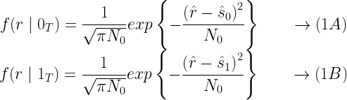
Assume that the BPSK symbols are transmitted through an AWGN channel characterized by variance = N0/2 Watts. When 0 is transmitted, the received symbol is represented by a Gaussian random variable ‘r‘ with mean=S0 = and variance =N0/2. When 1 is transmitted, the received symbol is represented by a Gaussian random variable – r with mean=S1= and variance =N0/2. Hence the conditional density function of the BPSK symbol (Figure 2) is given by,
Figure 1: BPSK – ideal constellation
Figure 2: Probability density function (PDF) for BPSK Symbols
An optimum receiver for BPSK can be implemented using a correlation receiver or a matched filter receiver (Figure 3). Both these forms of implementations contain a decision making block that decides upon the bit/symbol that was transmitted based on the observed bits/symbols at its input.
Figure 3: Optimum Receiver for BPSK
When the BPSK symbols are transmitted over an AWGN channel, the symbols appears smeared/distorted in the constellation depending on the SNR condition of the channel. A matched filter or that was previously used to construct the BPSK symbols at the transmitter. This process of projection is illustrated in Figure 4. Since the assumed channel is of Gaussian nature, the continuous density function of the projected bits will follow a Gaussian distribution. This is illustrated in Figure 5.
Figure 4: Role of correlation/Matched Filter
After the signal points are projected on the basis function axis, a decision maker/comparator acts on those projected bits and decides on the fate of those bits based on the threshold set. For a BPSK receiver, if the a-prior probabilities of transmitted 0’s and 1’s are equal (P=0.5), then the decision boundary or threshold will pass through the origin. If the apriori probabilities are not equal, then the optimum threshold boundary will shift away from the origin.
Figure 5: Distribution of received symbols
Considering a binary symmetric channel, where the apriori probabilities of 0’s and 1’s are equal, the decision threshold can be conveniently set to T=0. The comparator, decides whether the projected symbols are falling in region A or region B (see Figure 4). If the symbols fall in region A, then it will decide that 1 was transmitted. It they fall in region B, the decision will be in favor of ‘0’.
For deriving the performance of the receiver, the decision process made by the comparator is applied to the underlying distribution model (Figure 5). The symbols projected on the axis will follow a Gaussian distribution. The threshold for decision is set to T=0. A received bit is in error, if the transmitted bit is ‘0’ & the decision output is ‘1’ and if the transmitted bit is ‘1’ & the decision output is ‘0’.
This is expressed in terms of probability of error as,
Or equivalently,
By applying Bayes Theorem↗, the above equation is expressed in terms of conditional probabilities as given below,
Since a-prior probabilities are equal P(0T)= P(1T) =0.5, the equation can be re-written as
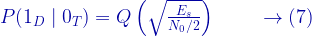
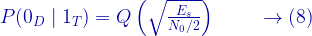
Intuitively, the integrals represent the area of shaded curves as shown in Figure 6. From the previous article, we know that the area of the shaded region is given by Q function.
Figure 6a, 6b: Calculating Error Probability
Similarly,
From (4), (6), (7) and (8),
For BPSK, since Es=Eb, the probability of symbol error (Ps) and the probability of bit error (Pb) are same. Therefore, expressing the Ps and Pb in terms of Q function and also in terms of complementary error function :
Rate this article: Note: There is a rating embedded within this post, please visit this post to rate it.
In simple words, The Q-function gives the probability that a random variable from a normal distribution will exceed a certain threshold value. The erf function gives the probability that a normally distributed variable will fall within a certain range.
Q function
Q functions are often encountered in the theoretical equations for Bit Error Rate (BER) involving AWGN channel. A brief discussion on Q function and its relation to erfc function is given here.
Gaussian process is the underlying model for an AWGN channel.The probability density function of a Gaussian Distribution is given by
Generally, in BER derivations, the probability that a Gaussian Random Variable \(X \sim N ( \mu, \sigma^2) \) exceeds \(x_0\) is evaluated as the area of the shaded region as shown in Figure 1.
Figure 1: Gaussian PDF and illustration of Q function
Mathematically, the area of the shaded region is evaluated as,
The above probability density function given inside the above integral cannot be integrated in closed form. So by change of variables method, we substitute
Here the function inside the integral is a normalized gaussian probability density function \(Y \sim N( 0, 1)\), normalized to mean \(\mu=0\) and standard deviation \(\sigma=1\).
The integral on the right side can be termed as Q-function, which is given by,
Thus Q function gives the area of the shaded curve with the transformation \(y = \frac{x-\mu}{\sigma}\) applied to the Gaussian probability density function. Essentially, Q function evaluates the tail probability of normal distribution (area of shaded area in the above figure).
The Q-function gives the probability that a random variable from a normal distribution will exceed a certain threshold value.
Error function
The complementary error function represents the area under the two tails of zero mean Gaussian probability density function of variance \(\sigma^2 = 1/2\). The error function gives the probability that the parameter lies outside that range.
The erf function gives the probability that a normally distributed variable will fall within a certain range.
Q function and Complementary Error Function (erfc)
From the limits of the integrals in equation (4) and (6) one can conclude that Q function is directly related to complementary error function (erfc). It follows from equation (4) and (6), Q function is related to complementary error function by the following relation.
Keep a note of the following equations that can come handy when deriving probability of bit errors for various scenarios. These equations are compiled here for easy reference.
If we have a normal variable \(X \sim N (\mu, \sigma^2)\), the probability that \(X > x\) is
\[\displaystyle{ Pr \left( X > x \right) = Q \left( \frac{x-\mu}{\sigma} \right ) } \quad\quad (10) \]
If we want to know the probability that \(X\) is away from the mean by an amount ‘a’ (on the left or right side of the mean), then
Application of Q function in computing the Bit Error Rate (BER) or probability of bit error will be the focus of our next article.
Applications
The Q-function and the error function (erf) are important mathematical functions that arise in many fields, including probability theory, statistics, signal processing, and communications engineering. Here are some reasons why these functions are important:
Probability calculations: The Q-function and erf function are used in probability calculations involving Gaussian distributions. The Q-function gives the probability that a random variable from a normal distribution will exceed a certain threshold value. The erf function gives the probability that a normally distributed variable will fall within a certain range.
Signal processing: In signal processing, the Q-function is used to calculate the probability of bit error in digital communication systems. This is important for designing communication systems that can reliably transmit data over noisy channels.
Statistical analysis: The Q-function and erf function are used in statistical analysis to model data and estimate parameters. For example, in hypothesis testing, the Q-function can be used to calculate p-values.
Mathematical modeling: The Q-function and erf function arise naturally in mathematical models for various phenomena. For example, the heat equation in physics and the Black-Scholes equation in finance both involve the erf function.
Computational efficiency: In some cases, the Q-function and erf function provide a more efficient and accurate way of calculating certain probabilities and integrals than other methods.
Key focus: Understand the basics of estimation theory with a simple example in communication systems. Know how to assess the performance of an estimator.
A simple estimation problem : DSB-AM receiver
In Double Side Band – Amplitude Modulation (DSB-AM), the desired message is amplitude modulated over a carrier of frequency f0. The following discussion is with reference to the figure 1. In the frequency domain, the spectrum of the message signal, which is a baseband signal, may look like the one shown in (a). After the modulation over a carrier frequency off0, the spectrum of the modulated signal will look like as shown in (b). The modulated signal has spectral components centered at f0 and -f0.
Figure 1: Illustrating estimation of unknowns f and Φ using DSB-AM receiver
The modulated signal is a function of three factors : 1) actual message – m(t) 2) carrier frequency – f0 3) phase uncertainty – Φ0
The modulated signal can be expressed as,
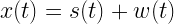
To simplify things, let’s consider that the modulated signal is passed via an ideal channel (no impairments added by the channel, so we can do away with channel equalization and other complex stuffs in the receiver). The modulated signal hits the antenna located at front end of our DSBC receiver. Usually the receiver front end is employed with a band-pass filter and amplifier to put the received signal in the desired band of operation & level, as expected by the receiver. The electronics in the front end receiver adds noise to the incoming signal (modeled as white noise – w(t) ). The signal after the BPF and amplifier combination is expressed as x(t), which is a combination of our desired signal s(t) and the front end noise w(t). Thus x(t) can be expressed as
The signal x(t) is band-pass (centered around the carrier frequency f0). To bring x(t) back to the baseband, a mixer is employed that multiplies x(t) with a tone centered at f0 (generated by a local oscillator). Actually a low pass filter is usually employed after the mixer, for extracting the desired signal at the baseband.
As the receiver has no knowledge about the carrier frequency, there must exist a technique/method to extract this information from the incoming signal x(t) itself. Not only the carrier frequency (f0) but also the phase Φ0 of the carrier need to be known at the receiver for proper demodulation. This leads us to the problem of “estimation”.
Estimation of unknown parameters
In “estimation” problem, we are confronted with estimating one or more unknown parameters based on a sequence of observed data. In our problem, the signal x(t) is the observed data and the parameters that are to be estimated are f0 and Φ0 .
Now, we add an estimation algorithm at the receiver, that takes in the signal x(t) and computes estimates of f0 and Φ0.The estimated values are denoted with a cap on their respective letters.The estimation algorithm can be simply stated as follows
Given , estimate and that are optimal in some sense.
So far, all the notations were expressed in continuous domain. To simplify calculations, let’s state the estimation problem in discrete time domain. In discrete time domain, the samples of observed signal – which is a combination of actual signal and noise is expressed As
The noise samples w[n] is a random variable, that randomizes every time we observe x[n]. Each time when we observe the “observed” samples – x[n] , we think of it as having the same “actual” signal samples – s[n] but with different realizations of the noise samples w[n]. Thus w[n] can be modeled as a Random Variable (RV). Since the underlying noise w[n] is a random variable, the estimates and that result from the estimation are also random variables.
Now the estimation algorithm can be stated as follows:
Given the observed data samples – x[n] = ( x[0], x[1],x[2], … ,x[N-1] ), our goal is to find estimator functions that maps the given data into estimates.
Assessing the performance of the estimation algorithm
Since the estimates and are random variables, they can be described by a probability density function (PDF). The PDF of the estimates depend on following factors :
1. Structure of s[n] 2. Probability model of w[n] 3. Form of estimation function g(x)
For example, the PDF of the estimate may take the following shape,
Figure 2: Probability Density function of estimate – f
The goal of the estimation algorithm is to give an estimate that is unbiased (mean of the estimate is equal to the actual f0) and has minimum variance. This criteria can be expressed as,
Same type of argument will hold for the other estimate :
Note: There is a rating embedded within this post, please visit this post to rate it.
In GMSK modulation (used in GSM and DECT standard), a GMSK signal is generated by shaping the information bits in NRZ format through a Gaussian Filter. The filtered pulses are then frequency modulated to yield the GMSK signal. GMSK modulation is quite insensitive to non-linearities of power amplifier and is robust to fading effects. But it has a moderate spectral efficiency.
An expression for the Gaussian Filter with 3dB Bandwidth is derived here.
The requirements for a gaussian filter used for GMSK modulation in GSM/DECT standard are as follows,
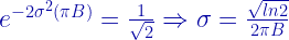
Now the challenge is to design a Gaussian Filter fG(t) that satifies the 3dB bandwidth requirement i.e. in the frequency domain at some frequency f=B, the filter should posses -3dB gain ( in otherwords => half power point located at f=B)
The expression for the required Gaussian Filter can be obtained by choosing the variance of the above mentioned distribution so that the Fourier Transform of the above mentioned expression has a -3dB power gain at f=B.
The fourier transform of the above mentioned expression is
A signal is a bandpass signal if we can fit all its frequency content inside a bandwidth . Bandwidth is simply the difference between the lowest and the highest frequency present in the signal.
“In order for a faithful reproduction and reconstruction of a bandpass analog signal with bandwidth – , the signal should be sampled at a Sampling frequency () that is greater than or equal to twice the maximum bandwidth of the signal:
Consider a bandpass signal extending from 150Hz to 200Hz. The bandwidth of this signal is . In order to faithfully represent the above signal in the digital domain the sampling frequency must be . Note that the sampling frequency 100Hz is far below the maximum content of the signal (which is 200Hz). That is why the bandpass sampling is also called “under-sampling”. As long as the sampling frequency is greater than or equal to twice the bandwidth of the signal, the reconstruction back to analog domain will be error free.
Going back to the aliasing zone figure, if the signal of interest is in the zone other than zone 1, it is called a bandpass signal and the sampling operation is called “Intermediate Sampling” or “Harmonic Sampling” or “Under Sampling” or “Bandpass Sampling”.
Folding Frequencies and Aliasing Zones
Note that zone 1 is a mirror image of zone 2 (with frequency reversal). Similarly zone 3 is a mirror image of zone 4 etc.., Also, any signal in zone 1 will be reflected in zone 2 with frequency reversal which inturn will be copied in zone 3 and so on.
Lets say the signal of interest lies in zone 2. This will be copied in all the other zones. Zone 1 also contains the sampled signal with frequency reversal which can be correct by reversing the order of FFT in digital domain.
No matter in which zone the signal of interest lies, zone 1 always contains the signal after sampling operation is performed. If the signal of interest lies in any of the even zones, zone 1 contains the sampled signal with frequency reversal. If the signal of interest lies in any of the odd zones, zone 1 contains the sampled signal without frequency reversal.
Example:
Consider an AM signal centered at carrier frequency 1MHz, with two components offset by 10KHz – 0.99 MHz and 1.01 MHz. So the AM signal contains three frequency components at 0.99 MHz, 1 MHz and 1.01 MHz.
Our desire is to sample the AM signal. As with the usual sampling theorem (baseband), we know that if we sample the signal at twice the maximum frequency i.e Fs>=2*1.01MHz=2.02 MHz there should be no problem in representing the analog signal in digital domain.
By the bandpass sampling theorem, we do not need to use a sampler running at Fs>=2.02 MHz. Faster sampler implies more cost. By applying the bandpass sampling theorem, we can use a slower sampler and reduce the cost of the system. The bandwidth of the signal is 1.01MHz-0.99 MHz = 20 KHz. So, just sampling at will convert the signal to digital domain properly and we can also avoid using an expensive high rate sampler (if used according to baseband sampling theorem).
Lets set the sampling frequency to be (which is 3 times higher than the minimum required sampling rate of 40KHz or oversampling rate =3).
Now we can easily find the position of the spectral components in the sampled output by using the aliasing zone figure as given above. Since , will be 60KHz. So the zone 1 will be from 0 to 60 KHz, zone 2 -> 60-120KHz and so on. The three spectral components at 0.99MHz, 1MHz and 1.01 MHz will fall at zone 17 ( how ? 0.99 MHz/60 KHz = 16.5 , 1MHz/60KHz = 16.67 and 1.01MHz/60KHz = 16.83 , all figures approximating to 17). By the aliasing zone figure, zone 16 contains a copy of zone 17, zone 15 contains a copy of zone 16, zone 14 contains a copy of zone 15 and so on… Finally zone 1 contains the copy of zone 2 (Frequency reversal also exist at even zones). In effect, zone 1 contains a copy of zone 17. Since the original spectral components are at zone 17, which is an odd zone, zone 1 contains the copy of spectral components at zone 17 without frequency reversal.
Since there is no frequency reversal, in zone 1 the three components will be at 30KHz, 40KHz and 50KHz (You can easily figure this out ).
This operation has downconverted our signal from zone 17 to zone 1 without distorting the signal components. The downconverted signal can be further processed by using a filter to select the baseband downconverted components. Following figure illustrates the concept of bandpass sampling.
Bandpass Sampling
Consider the same AM signal with three components at 0.99MHz, 1MHz and 1.01 MHz. Now we also have an “unwanted” fourth component at 1.2 MHz along with the incoming signal. If we sample the signal at 120 KHz, it will cause aliasing (because the bandwidth of the entire signal is 1.2-0.99 = 0.21 MHz = 210 KHz and the sampling frequency of 120KHz is below twice the bandwidth). In order to avoid anti-aliasing and to discard the unwanted component at 1.2 MHz, an anti-aliasing bandpass filter has to be used to select those desired component before performing the sampling operation at 120KHz. This is also called “pre-filtering”. The following figure illustrates this concept.
“Nyquist-Shannon Sampling Theorem” is the fundamental base over which all the digital processing techniques are built. Processing a signal in digital domain gives several advantages (like immunity to temperature drift, accuracy, predictability, ease of design, ease of implementation etc..,) over analog domain processing.
Analog to Digital conversion:
In analog domain, the signal that is of concern is continuous in both time and amplitude. The process of discretization of the analog signal in both time domain and amplitude levels yields the equivalent digital signal. The conversion of analog to digital domain is a three step process 1) Discretization in time – Sampling 2) Discretization of amplitude levels – Quantization 3) Converting the discrete samples to digital samples – Coding/Encoding
Components of ADC
The sampling operation samples (“chops”) the incoming signal at regular interval called “Sampling Rate” (denoted by ). Sampling Rate is determined by Sampling Frequency (denoted by ) as Lets consider the following logical questions: * Given a real world signal, how do we select the sampling rate in order to faithfully represent the signal in digital domain ? * Is there any criteria for selecting the sampling rate ? * Will there be any deviation if the signal is converted back to analog domain ? Answer : Consult the “Nyquist-Shannon Sampling Theorem” to select the sampling rate or sampling frequency.
Nyquist-Shannon Sampling Theorem:
The following sampling theorem is the exact reproduction of text from Shannon’s classic paper[1],
“If a function f(t) contains no frequencies higher than W cps, it is completely determined by giving its ordinates at a series of points spaced 1/2W seconds apart.”
Sampling Theorem mainly falls into two categories : 1) Baseband Sampling – Applied for signals in the baseband (useful frequency components extending from 0Hz to some Fm Hz) 2) Bandpass Sampling – Applied for signals whose frequency components extent from some F1 Hz to F2Hz (where F2>F1) In simple terms, the Nyquist Shannon Sampling Theorem for Baseband can be explained as follows
Baseband Sampling:
If the signal is confined to a maximum frequency of Fm Hz, in other words, the signal is a baseband signal (extending from 0 Hz to maximum Fm Hz).
In order for a faithful reproduction and reconstruction of an analog signal that is confined to a maximum frequency Fm, the signal should be sampled at a Sampling frequency (Fs) that is greater than or equal to twice the maximum frequency of the signal:
Consider a 10Hz sine wave in analog domain. The maximum frequency present in this signal is Fm=10 Hz (obviously no doubt about it !!!). Now, to satisfy the sampling theorem that is stated above and to have a faithful representation of the signal in digital domain, the sampling frequency can be chosen as Fs >=20Hz. That is, we are free to choose any number above 20 Hz. Higher the sampling frequency higher is the accuracy of representation of the signal. Higher sampling frequency also implies more samples, which implies more storage space or more memory requirements. In time domain, the process of sampling can be viewed as multiplying the signal with a series of pulses (“pulse train) at regular interval – Ts. In frequency domain, the output of the sampling process gives the following components – Fm (original frequency content of the signal), Fs±Fm,2Fs±Fm,3Fs±Fm,4Fs±Fm and so on and on…
Baseband Sampling
Now the sampled signal contains lots of unwanted frequency components (Fs±Fm,2Fs±Fm,…). If we want to convert the sampled signal back to analog domain, all we need to do is to filter out those unwanted frequency components by using a “reconstruction” filter (In this case it is a low pass filter) that is designed to select only those frequency components that are upto Fm Hz. The above process mentions only the sampling part which samples the incoming analog signal at regular intervals. Actually a quantizer will follow the sampler which will discretize (“quantize”) amplitude levels of the sampled signal. The quantized amplitude levels are sent to an encoder that converts the discrete amplitude levels to binary representation (binary data). So when converting the binary data back to analog domain, we need a Digital to Analog Converter (DAC) that converts the binary data to analog signal. Now the converted signal after the DAC contains the same unwanted frequencies as well as the wanted component. Thus a reconstruction filter with proper cut-off frequency has to placed after the DAC to filter out only the wanted components.
Aliasing and Anti-aliasing:
Consider a signal with two frequency components f1=10Hz – which is our desired signal and f2=20Hz – which is a noise. Let’s say we sample the signal at 30Hz. The first frequency component f1=10Hz will generate following frequency components at the output of the multiplier (sampler) – 10Hz,20Hz,40Hz,50Hz,70Hz and so on. The second frequency component f2=20Hz will generate the following frequency components at the output of the multiplier – 20Hz,10Hz,50Hz,40Hz,80Hz and so on…
Aliasing and Anti-aliasing
Note the 10Hz component that is generated by f2=20Hz. This 10Hz component (which is a manifestation of noisy component f2=20Hz) will interfere with our original f1=10Hz component and are indistinguishable. This 10Hz component is called “alias” of the original component f2=20Hz (noise). Similarly the 20Hz component generated by f1=10Hz component is an “alias” of f1=10Hz component. This 20Hz alias of f1=10Hz will interfere with our original component f2=20Hz and are indistinguishable. We do not need to care about the interference that occurs at 20Hz since it is a noise and any way it has to be eliminated. But we need to do something about the aliasing component generated by the f2=20Hz. Since this is a noise component, the aliasing component generated by this noise will interfere with our original f1=10Hz component and will corrupt it. Aliasing depends on the sampling frequency and its relationship with the frequency components. If we sample a signal at Fs, all the frequency components from Fs/2 to Fs will be alias of frequency components from 0 to Fs/2 and vice versa. This frequency – Fs/2 is called “Folding frequency” since the frequency components from Fs/2 to Fs folds back itself and interferes with the components from 0Hz to Fs/2 Hz and vice versa. Actually the aliasing zones occur on the either sides of 0.5Fs, 1.5Fs, 2.5Fs,3.5Fs etc… All these frequencies are also called “Folding Frequencies” that causes frequency reversal. Similarly aliasing also occurs on either side of Fs,2Fs,3Fs,4Fs… without frequency reversals. The following figure illustrates the concept of aliasing zones.
Folding Frequencies and Aliasing Zones
In the above figure, zone 2 is just a mirror image of zone 1 with frequency reversal. Similarly zone 2 will create aliases in zone 3 (without frequency reversal), zone 3 creates mirror image in zone 4 with frequency reversal and so on… In the example above, the folding frequency was at Fs/2=15Hz, so all the components from 15Hz to 30Hz will be the alias of the components from 0Hz to 15Hz. Once the aliasing components enter our band of interest, it is impossible to distinguish between original components and aliased components and as a result, the original content of the signal will be lost. In order to prevent aliasing, it is necessary to remove those frequencies that are above Fs/2 before sampling the signal. This is achieved by using an “anti-aliasing” filter that precedes the analog to digital converter. An anti-aliasing filter is designed to restrict all the frequencies above the folding frequency Fs/2 and therefore avoids aliasing that may occur at the output of the multiplier otherwise.
A complete design of ADC and DAC
Thus, a complete design of analog to digital conversion contains an anti-aliasing filter preceding the ADC and the complete design of digital to analog conversion contains a reconstruction filter succeeding the DAC.
ADC and DAC chain
Note: Remember that both the anti-aliasing and reconstruction filters are analog filters since they operate on analog signal. So it is imperative that the sampling rate has to be chosen carefully to relax the requirements for the anti-aliasing and reconstruction filters.
Effects of Sampling Rate:
Consider a sinusoidal signal of frequency Fm=2MHz. Lets say that we sample the signal at Fs=8MHz (Fs>=2*Fm). The factor Fs/Fm is called “over-sampling factor”. In this case we are over-sampling the signal by a factor of Fm=8MHz/2MHz = 4. Now the folding frequency will be at Fs/2 = 4MHz. Our anti-aliasing filter has to be designed to strictly cut off all the frequencies above 4MHz to prevent aliasing. In practice, ideal brick wall response for filters is not possible. Any filter will have a transition band between pass-band and stop-band. Sharper/faster roll off transition band (or narrow transition band) filters are always desired. But such filters are always of high orders. Since both the anti-aliasing and reconstruction filters are analog filters, high order filters that provide faster roll-off transition bands are expensive (Cost increases proportionally with filter order). The system also gets bulkier with increase in filter order.Therefore, to build a relatively cheaper system, the filter requirement in-terms of width of the transition band has to be relaxed. This can be done by increasing the sampling rate or equivalently the over-sampling factor. When the sampling rate (Fs) is increased, the distance between the maximum frequency content Fm and Fs/2 will increase. This increase in the gap between the maximum frequency content of the signal and Fs/2 will ease requirements on the transition bands of the anti-aliasing analog filter. Following figure illustrates this concept. If we use a sampling frequency of Fs=8MHz (over-sampling factor = 4), the transition band is narrower and it calls for a higher order anti-aliasing filter (which will be very expensive and bulkier). If we increase the sampling frequency to Fs=32MHz (over-sampling factor = 32MHz/2MHz=16), the distance between the desired component and Fs/2 has greatly increased that it facilitates a relatively inexpensive anti-aliasing filter with a wider transition band. Thus, increasing the sampling rate of the ADC facilitates simpler lower order anti-aliasing filter as well as reconstruction filter. However, increase in the sampling rate calls for a faster sampler which makes ADC expensive. It is necessary to compromise and to strike balance between the sampling rate and the requirement of the anti-aliasing/reconstruction filter.
Effects of Sampling Rate
Application : Up-conversion
In the above examples, the reconstruction filter was conceived as a low pass filter that is designed to pass only the baseband frequency components after reconstruction. Remember that any frequency component present in zone 1 will be reflected in all the zones (with frequency reversals in even zones and without frequency reversals in odd zones). So, if we design the reconstruction filter to be a bandpass filter selection the reflected frequencies in any of the zones expect zone 1, then we achieve up-conversion. In any communication system, the digital signal that comes out of a digital signal processor cannot be transmitted across as such. The processed signal (which is in the digital domain) has to be converted to analog signal and the analog signal has to be translated to appropriate frequency of operation that fits the medium of transmission. For example, in an RF system, a baseband signal is converted to higher frequency (up-conversion) using a multiplier and oscillator and then the high frequency signal is transmitted across the medium. If we have a band-pass reconstruction filter at the output of the DAC, we can directly achieve up-conversion (which saves us from using a multiplier and oscillator). The following figure illustrates this concept.
Goal: Simulate discrete-time cyclic-prefixed OFDM communication system. Explain role of IFFT/FFT, cyclic prefix. Simulate M-QPSK / M-QAM based cyclic prefixed OFDM over AWGN channel.
The schematic diagram of a simplified cyclic-prefixed OFDM (CP-OFDM) data transmission system is shown in Figure 1. The basic parameter to describe an OFDM system is to specify the number of subchannels () required to send the data. The number of subchannels is typically set to powers of 2, such as . The size of inverse discrete Fourier transform (IDFT) and discrete Fourier transform (DFT) need to be set accordingly.
The transmission begins by converting the source information stream into parallel subchannels. For convenience, the information stream is already represented as a symbol from the set . The data symbol in each subchannel is modulated using the chosen modulation technique such as MPSK or MQAM.
Since this is a baseband discrete-time model, where the signals are represented at symbol sampling instants, the information symbol on each parallel stream is assumed to be modulating a single orthogonal carrier. At this juncture, the modulated symbols on the parallel streams can be visualized as coming from different orthogonal subchannels in the frequency domain. The components of the orthogonal subchannels in the frequency domain are converted to time domain using IDFT operation.
Figure 1: Discrete-time simulation model for OFDM transmission and reception
The following generic function implements the modulation mapper (constellation mapping) shown in the Figure 1. The function supports MPSK modulation for and MQAM modulation that has square constellation : . It is built over the mpsk_modulator.m and mqam_modulator.m functions given in sections 5.3.2 and 5.3.3 of chapter 5 (Refer the book Wireless communication systems using Matlab).
modulation_mapper.m: Implementing the modulation mapper for MPSK and MQAM
function [X,ref]=modulation_mapper(MOD_TYPE,M,d)
%Modulation mapper for OFDM transmitter
% MOD_TYPE - 'MPSK' or 'MQAM' modulation
% M - modulation order, For BPSK M=2, QPSK M=4, 256-QAM M=256 etc..,
% d - data symbols to be modulated drawn from the set {1,2,...,M}
%returns
% X - modulated symbols
% ref -ideal constellation points that could be used by IQ detector
if strcmpi(MOD_TYPE,'MPSK'),
[X,ref]=mpsk_modulator(M,d);%MPSK modulation
else
if strcmpi(MOD_TYPE,'MQAM'),
[X,ref]=mqam_modulator(M,d);%MQAM modulation
else
error('Invalid Modulation specified');
end
end;end
OFDM signal is a composite signal that contains information from subchannels. Since the modulated symbols are visualized to be in frequency domain, it is converted to time-domain using IDFT. In the receiver, the corresponding inverse operation is performed by the DFT block. The IDFT and DFT blocks in the schematic can also be interchanged and it has no impact to the transmission.
In a time-dispersive channel, the orthogonality of the subcarriers cannot be maintained in a perfect state due to delay distortion. This problem is addressed by adding a cyclic extension (also called cyclic prefix) to the OFDM symbol (reference [1]). A cyclic extension is added by copying the last symbols from the vector and pasting it to its front as shown in Figure 2.
Figure 2: Adding a cyclic prefix in CP-OFDM
Cyclic extension of OFDM symbol converts the linear convolution channel to a channel performing cyclic convolution (view demo here) and this ensures orthogonality of subcarriers in a time-dispersive channel. It also completely eliminates the subcarrier interference as long as the impulse response of the channel is shorter than the cyclic prefix. At the receiver, the added cyclic prefix is simply removed from the received OFDM symbol.
On the receiver side, the demapper for demodulating MPSK and MQAM can be implemented by using a simple IQ detector that uses the minimum euclidean distance metric for demodulation. (discussion and function definitions in section 5.4.4 of chapter 5 (Refer the book Wireless communication systems using Matlab).
Performance of MPSK-CP-OFDM and MQAM-CP-OFDM on AWGN channel
The code (given in the book Wireless communication systems using Matlab) puts together all the functional blocks of an OFDM transmission system, that were described here, to simulate the performance of a CP-OFDM system over an AWGN channel. The code supports two types of underlying modulations for OFDM – MPSK or MQAM. It generates random data symbols, modulates them using the chosen modulation type, converts the modulated symbols to frequency domain using IDFT operation and adds cyclic prefix to form an OFDM symbol. The resulting OFDM symbols are then added with AWGN noise vector that corresponds to the specified value (AWGN noise model is described in this article).
On the receiver side, cyclic prefix is removed from the received OFDM symbol, DFT is performed and then the symbols are sent through a demapper for getting an estimate of the source symbols. The demapper is implemented by using a simple IQ detector that uses the minimum euclidean distance metric for demodulation. Finally, the symbol error rates are computed and compared against the theoretical symbol error rate curves for the respective modulations over AWGN. Simulated performance results are plotted in Figure 3.
Note: There is a rating embedded within this post, please visit this post to rate it.
Consider a non-ideal channel h(t)≠δ(t), that causes delay dispersion. Delay dispersion manifests itself as Inter Symbol Interference (ISI)on each subcarrier channel due to pulse overlapping. It will also cause ICC (Inter Carrier Interference ) due to the non-orthogonality of the received signal. Adding cyclic prefix to each OFDM symbol mitigates the problems of ISI and ICC by removing them altogether.
Lets say, without cyclic prefix we transmit the following N values (N=Nfft=length of FFT/IFFT) for a single OFDM symbol.
$$ X_0,X_1,X_2,…,X_{N-1} $$
Lets consider a cyclic prefix of length Ncp, ( where Ncp<N ), is formed by copying the last Ncp values from the above vector of X and adding those Ncp values to the front part of the same X vector.With a cyclic prefix length Ncp, ( where Ncp<N ), the following values constitute a single OFDM symbol :
If T is the duration of the an OFDM symbol in secs, due to the addition of cyclic prefix of length Ncp, the total duration of an OFDM symbol becomes T+Tcp, where Tcp=Ncp*T/N. Therefore, the number of samples allocated for cyclic prefix can be calculated as Ncp=Tcp*N/T, where N is the FFT/IFFT length, T is the IFFT/FFT period and Tcp is the duration of cyclic prefix.
The key ideas behind adding cyclic prefix :
1) Convert linear convolution in to circular convolution which eases the process of detecting the received signal by using a simple single tap equalizer
If you wish to know how the addition of cyclic prefix converts linear convolution to circular convolution, visit this link
2) Help combat ISI and ICC.
When a cyclic prefix of length Ncp is added to the OFDM symbol, the output of the channel (r) is given by circular convolution of channel impulse response (h) and the OFDM symbols with cyclic prefix (x).
$$ r=h \circledast x $$
As we know, for the discrete signals, circular convolution in the time domain translates to multiplication in the frequency domain.Thus, in frequency domain, the above equation translates to
$$ R=HX $$
At the receiver, R is the received signal (in Frequency domain) and our goal is to estimate the transmitted signal (X) from the received signal R. From the above equation, the problem of detecting the transmitted signal at the receiver side translate to a simple equalization equation as follows
$$ \hat{X}= \frac{R}{H} $$
After the FFT performed at the receiver side (i.e. after the FFT block in the receiver side), a single tap equalizer (which essentially implements the above equation) is used to estimate the transmitted OFDM symbol. It also corrects the phase and equalizes the amplitude.
A basic OFDM architecture with Cyclic Prefix is given below. (In the following diagram, symbols represented by small case letters are assumed to be in time domain, whereas the symbols represented by uppercase letters are assumedto be in frequency domain)
An OFDM communication Architecture with Cyclic Prefix
The IEEE specs specify the length of the Cyclic prefix in terms of its duration.
Lets see how to convert the specified duration (Tcp) in to actual number of samples assigned for cyclic prefix (Ncp).
Lets see an example of deriving Ncp from IEEE 802.11 spec [1]
Given parameters in the spec:
N=64;                           %FFT size or total number of subcarriers (used + unused) 64
Nsd = 48;                      %Number of data subcarriers 48
Nsp = 4 ;                        %Number of pilot subcarriers 4
ofdmBW = 20 * 10^6 ;  % OFDM bandwidth

Derived Parameters:
deltaF = ofdmBW/N;      % Bandwidth for each subcarrier - include all used and unused subcarries
Tfft = 1/deltaF;               % IFFT or FFT period = 3.2us
Tgi = Tfft/4;                    % Guard interval duration - duration of cyclic prefix - 1/4th portion of OFDM symbols
Tsignal = Tgi+Tfft;          % Total duration of BPSK-OFDM symbol = Guard time + FFT period
Ncp = N*Tgi/Tfft;           %Number of symbols allocated to cyclic prefix
Nst = Nsd + Nsp;           % Number of total used subcarriers
nBitsPerSym=Nst;           %For BPSK the number of Bits per Symbol is same as number of subcarriers
In the previous article, the architecture of an OFDM transmitter was described using sinusoidal components. Generally, an OFDM signal can be represented as
\[OFDM\; signal = c(t)=\sum_{n=0}^{N-1}s_{n}(t)sin(2\pi f_{n}t )\]
\(s(t)\) = symbols mapped to chosen constellation (BPSK/QPSK/QAM etc..,)
\(f_n\) = orthogonal frequency
This equation can be thought of as an IFFT process ( Inverse Fast Fourier Transform). The Fourier transform breaks a signal into different frequency bins by multiplying the signal with a series of sinusoids. This essentially translates the signal from time domain to frequency domain. But, we always view IFFT as a conversion process from frequency domain to time domain.
FFT is represented by
\[X(k)=\sum_{n=0}^{N-1}x(n) \cdot sin \left(\frac{2\pi kn}{N} \right)+j\sum_{n=0}^{N-1}x(n) \cdot cos \left(\frac{2\pi kn}{N} \right)\]
\[x(n)=\sum_{n=0}^{N-1}X(k) \cdot sin \left(\frac{2\pi kn}{N} \right)-j\sum_{n=0}^{N-1}X(k) \cdots cos \left(\frac{2\pi kn}{N} \right)\]
where as its dual , IFFT is given by
The equation for FFT and IFFT differ by the co-efficients they take and the minus sign. Both equation does the same thing. They multiply the incoming signal with a series of sinusoids and separates them into bins.In fact, FFT and IFFT are dual and behaves in a similar way.IFFT and FFT blocks are interchangeable.
Since the OFDM signal ( c(t) in the equation above ) is in time domain, IFFT is the appropriate choice to use in the transmitter, which can be thought of as converting frequency domain samples to time domain samples. Well, you might ask : s(t) is not in frequency domain and they are already in time domain; so whats the need to convert it into time domain again ? The answer is IFFT/FFT equation comes handy in implementing the conversion process and we can eliminate the individual sinusoidal multipliers required in the transmitter/receiver side. The following figure illustrates, how the use of IFFT in the transmitter eliminates the need for separate sinusoidal converters. Always remember that IFFT and FFT blocks in the transmitter are interchangeable as long as their duals are used in receiver.
OFDM implementation using FFT and IFFT
The entire architecture of a basic OFDM system with both transmitter and receiver will look like this
A Complete OFDM communication system
An OFDM system is defined by IFFT/FFT length – N ,the underlying modulation technique ( BPSK/QPSK/QAM), supported data rate, etc..,. The FFT/IFFT length N defines the number of total subcarriers present in the OFDM system. For example, an OFDM system with N=64 provides 64 subcarriers. In reality, not all the subcarriers are utilized for data transmission. Some subcarriers are reserved for pilot carriers (used for channel estimation/equalization and to combat magnitude and phase errors in the receiver) and some are left unused to act as guard band. OFDM system do not transmitany data on the subcarriers that are near the two ends of the transmission band ( Not necessarily at the ends of the bands, implementation may differ). These subcarriers are collectively called guard band. The reservation of subcarriers to guard bands helps to reduce the out of band radiation and thus eases the requirements on transmitter front-end filters.The subcarriers in the guard band are also called Null subcarriers or virtual subcarriers.
For example IEEE 802.11 standard[1]specifies the following parameters for its OFDM physical layer.
FFT/IFFT size = 64 ( implies 64 subcarriers in total = used + unused = N_{fft})
Number of data subcarriers = 48 (\( N_d\))
Number of pilot subcarriers = 4 (\(N_p\))
Derived parameters from the above specification.
Number of total USED subcarriers = 52 (\( N_u = N_d+ N_p \))
Number of total UNUSED subcarriers = 12 (\( N_{un} = N_{fft} – N_u\)).
According to the spec, these 52 used subcarriers are distributed in the following way. The 52 used subcarriers are named as 1,2,3,…,26 and -1,-2,-3,…,-26. The used subcarriers 1 to 26 are mapped to 1 to 26 of IFFT inputs and the subcarriers -1,-2,..,-26 are mapped to the IFFT inputs 38 to 63. The remaining IFFT inputs 27 to 37 and the input 0 (dc input) are set to 0 .In this manner the 12 null subcarriers are mapped to IFFT inputs.
This website uses cookies to improve your experience while you navigate through the website. Out of these, the cookies that are categorized as necessary are stored on your browser as they are essential for the working of basic functionalities of the website. We also use third-party cookies that help us analyze and understand how you use this website. These cookies will be stored in your browser only with your consent. You also have the option to opt-out of these cookies. But opting out of some of these cookies may affect your browsing experience.
Necessary cookies are absolutely essential for the website to function properly. These cookies ensure basic functionalities and security features of the website, anonymously.
Cookie
Duration
Description
cookielawinfo-checbox-analytics
11 months
This cookie is set by GDPR Cookie Consent plugin. The cookie is used to store the user consent for the cookies in the category "Analytics".
cookielawinfo-checbox-analytics
11 months
This cookie is set by GDPR Cookie Consent plugin. The cookie is used to store the user consent for the cookies in the category "Analytics".
cookielawinfo-checbox-functional
11 months
The cookie is set by GDPR cookie consent to record the user consent for the cookies in the category "Functional".
cookielawinfo-checbox-functional
11 months
The cookie is set by GDPR cookie consent to record the user consent for the cookies in the category "Functional".
cookielawinfo-checbox-others
11 months
This cookie is set by GDPR Cookie Consent plugin. The cookie is used to store the user consent for the cookies in the category "Other.
cookielawinfo-checbox-others
11 months
This cookie is set by GDPR Cookie Consent plugin. The cookie is used to store the user consent for the cookies in the category "Other.
cookielawinfo-checkbox-necessary
11 months
This cookie is set by GDPR Cookie Consent plugin. The cookies is used to store the user consent for the cookies in the category "Necessary".
cookielawinfo-checkbox-performance
11 months
This cookie is set by GDPR Cookie Consent plugin. The cookie is used to store the user consent for the cookies in the category "Performance".
viewed_cookie_policy
11 months
The cookie is set by the GDPR Cookie Consent plugin and is used to store whether or not user has consented to the use of cookies. It does not store any personal data.
Functional cookies help to perform certain functionalities like sharing the content of the website on social media platforms, collect feedbacks, and other third-party features.
Performance cookies are used to understand and analyze the key performance indexes of the website which helps in delivering a better user experience for the visitors.
Analytical cookies are used to understand how visitors interact with the website. These cookies help provide information on metrics the number of visitors, bounce rate, traffic source, etc.


![x[n] = s[n;f_0, \phi_0] + w[n]](https://s0.wp.com/latex.php?latex=x%5Bn%5D+%3D+s%5Bn%3Bf_0%2C+%5Cphi_0%5D+%2B+w%5Bn%5D+&bg=ffffff&fg=000&s=2&c=20201002)

![\hat{f}_{0}=g_{1}(x[0], x[1],x[2],\cdots,x[N-1])=g_{1} \left( \textbf{x} \right)](https://s0.wp.com/latex.php?latex=%5Chat%7Bf%7D_%7B0%7D%3Dg_%7B1%7D%28x%5B0%5D%2C+x%5B1%5D%2Cx%5B2%5D%2C%5Ccdots%2Cx%5BN-1%5D%29%3Dg_%7B1%7D+%5Cleft%28+%5Ctextbf%7Bx%7D+%5Cright%29+&bg=ffffff&fg=000&s=2&c=20201002)

![\hat{\phi}_{0} = g_{2} (x[0], x[1], x[2], \cdots, x[N-1]) = g_{2} \left( \textbf{x} \right)](https://s0.wp.com/latex.php?latex=%5Chat%7B%5Cphi%7D_%7B0%7D+%3D+g_%7B2%7D+%28x%5B0%5D%2C+x%5B1%5D%2C+x%5B2%5D%2C+%5Ccdots%2C+x%5BN-1%5D%29+%3D+g_%7B2%7D+%5Cleft%28+%5Ctextbf%7Bx%7D+%5Cright%29+&bg=ffffff&fg=000&s=2&c=20201002)


![\begin{aligned} E\left\{\hat{f}_0 \right\} &= f_0 \\ \sigma^{2}_{\hat{f}_0} &= E \left\{ \left( \hat{f}_0 - E [ \hat{f}_0] \right)^2 \right\} \quad \text{should be minimum} \end{aligned}](https://s0.wp.com/latex.php?latex=%5Cbegin%7Baligned%7D+E%5Cleft%5C%7B%5Chat%7Bf%7D_0+%5Cright%5C%7D+%26%3D+f_0+%5C%5C+%5Csigma%5E%7B2%7D_%7B%5Chat%7Bf%7D_0%7D+%26%3D+E+%5Cleft%5C%7B+%5Cleft%28+%5Chat%7Bf%7D_0+-+E+%5B+%5Chat%7Bf%7D_0%5D+%5Cright%29%5E2+%5Cright%5C%7D+%5Cquad+%5Ctext%7Bshould+be+minimum%7D+%5Cend%7Baligned%7D+&bg=ffffff&fg=000&s=2&c=20201002)


![F[f(t)]=e^{-2 \sigma^{2} ( \pi f) }](https://s0.wp.com/latex.php?latex=F%5Bf%28t%29%5D%3De%5E%7B-2+%5Csigma%5E%7B2%7D+%28+%5Cpi+f%29+%7D&bg=ffffff&fg=0000A0&s=2&c=20201002)