Methods to compute linear convolution

Mathematical details of convolution, its relationship to polynomial multiplication and the application of Toeplitz matrices in computing linear convolution are discussed in the previous article. A short survey of different techniques to compute discrete linear convolution (with Matlab code) is given here. Definition Given an LTI (Linear Time Invariant) system with impulse response \(h[n]\) and … Read more

White Noise : Simulation and Analysis using Matlab

Definition A random process (or signal for your visualization) with a constant power spectral density (PSD) function is a white noise process. Power Spectral Density Power Spectral Density function (PSD) shows how much power is contained in each of the spectral component. For example, for a sine wave of fixed frequency, the PSD plot will … Read more

Symbol Timing Recovery for QPSK (digital modulations)

The goal of timing recovery is to estimate and correct the sampling instants and phase at the receiver, such that it allows the receiver to decode the transmitted symbols reliably. What is Symbol timing Recovery : When transmitting data across a communication system, three things are important: frequency of transmission, phase information and the symbol … Read more

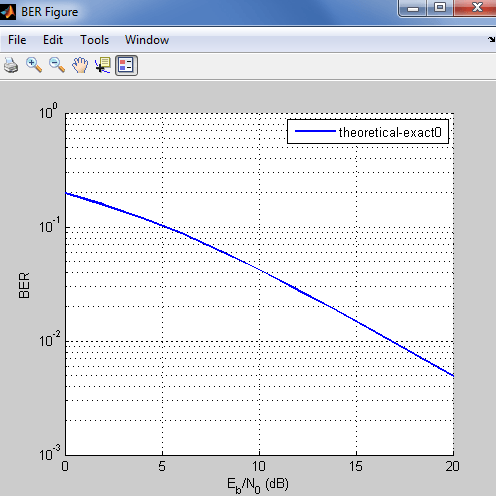
Theoretical BER using Matlab – BERTOOL

When simulating digital modulations in Matlab, it is useful to verify the simulated BER performance curves against theoretical BER curves.Matlab has an inbuilt visualization tool, ‘BERTOOL’, for this purpose. Matlab’s BERTOOL supports 6 types of digital modulations over 3 types of channel for plotting theoretical BER. The six supported modulations are PSK,DPSK,OQPSK,PAM,QAM,FSK and the three … Read more

Tips & Tricks : Indexing in Matlab

Let’s review indexing techniques in Matlab: Indexing one dimensional array, two dimensional array, logical indexing, reversiong a vector – are covered. Consider a sample vector in Matlab. Index with single value Index with range of values Select a range of elements using ‘:’ operator. Example: Select elements with index ranging from 1 to 5. Making … Read more

Cholesky decomposition: Python & Matlab

Cholesky decomposition is an efficient method for inversion of symmetric positive-definite matrices. Let’s demonstrate the method in Python and Matlab. Cholesky factor Any symmetric positive definite matrix can be factored as where is lower triangular matrix. The lower triangular matrix is often called “Cholesky Factor of ”. The matrix can be interpreted as square root … Read more

Natural Binary Codes and Gray Codes

In a given communication system, we always want to send data that represent real world data representing some physical quantity (be it speech, temperature, etc..,) .The real world physical quantity exist in analog domain and it becomes imperative to convert it to digital domain if we want to send it via a digital communication system. … Read more

MPSK modulation: simulate in Matlab & Python

A generic complex baseband simulation technique, to simulate all M-ary phase shift keying (M-PSK) modulation techniques is given here. The given simulation code is very generic, and it plots both simulated and theoretical symbol error rates for all MPSK modulation techniques. M-ary phase shift keying (M-PSK) modulation In phase shift keying, all the information gets … Read more

Eb/N0 Vs BER for BPSK over Rayleigh Channel and AWGN Channel

The phenomenon of Rayleigh Flat fading and its simulation using Clarke’s model and Young’s model were discussed in the previous posts. The performance (Eb/N0 Vs BER) of BPSK modulation (with coherent detection) over Rayleigh Fading channel and its comparison over AWGN channel is discussed in this post. We first investigate the non-coherent detection of BPSK … Read more

Simulation of Rayleigh Fading ( Clarke’s Model – sum of sinusoids method)

A multipath fading channel  can be modeled as a FIR (Finite Impulse Response) filter with the following impulse response. $$ h( \tau ; t ) = h_{0}(t) \delta ( \tau – \tau_{0}(t)) + h_{1}(t) \delta ( \tau – \tau_{1}(t)) + . . . + h_{L-1}(t) \delta ( \tau – \tau_{L-1}(t)) $$ where h(τ,t) is the … Read more