Let’s learn the equations and the filter model for simulating square root raised cosine (SRRC) pulse shaping. Before proceeding, I urge you to read about basics of pulse shaping in this article.


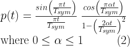
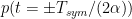
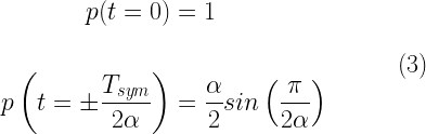
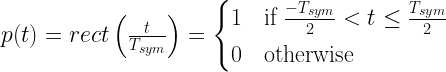
Raised-cosine pulse shaping filter is generally employed at the transmitter. Let


If the receive filter is matched with the transmit filter, we have


Thus, the transmit and the receive filter take the form


with


This article is part of the book |
The roll-of factor for the SRRC is denoted as


A function for generating SRRC pulse shape is given next. It is followed by a test code that plots the combined impulse response of transmit-receive SRRC filter combination and also plots the frequency domain view of a single SRRC pulse as shown in Figure 1
The combined impulse response matters, as we can identify that the combined response hits zero at symbol sampling instants. This indicates that the job of ISI cancellation is split between transmitter and receiver filters. Note that the combined impulse response of two SRRC filters is same as the impulse response of the RC filter.
Program 1: srrcFunction.m: Function for generating square-root raised-cosine pulse (click here)
Program 2: test_SRRCPulse.m: Square-root raised-cosine pulse characteristics
Tsym=1; %Symbol duration in seconds
L=10; % oversampling rate, each symbol contains L samples
Nsym = 80; %filter span in symbol durations
betas=[0 0.22 0.5 1];%root raised-cosine roll-off factors
Fs=L/Tsym;%sampling frequency
lineColors=['b','r','g','k','c']; i=1;legendString=cell(1,4);
for beta=betas %loop for various alpha values
	[srrcPulseAtTx,t]=srrcFunction(beta,L,Nsym); %SRRC Filter at Tx
	srrcPulseAtRx = srrcPulseAtTx;%Using the same filter at Rx
	%Combined response matters as it hits 0 at desired sampling instants
	combinedResponse = conv(srrcPulseAtTx,srrcPulseAtRx,'same');

	subplot(1,2,1); t=Tsym*t; %translate time base & normalize reponse
	plot(t,combinedResponse/max(combinedResponse),lineColors(i));
	hold on;

	%See Chapter 1 for the function 'freqDomainView'
	[vals,F]=freqDomainView(srrcPulseAtTx,Fs,'double');
	subplot(1,2,2);
	plot(F,abs(vals)/abs(vals(length(vals)/2+1)),lineColors(i));
	hold on;legendString{i}=strcat('\beta =',num2str(beta) );i=i+1;
end
subplot(1,2,1);
title('Combined response of SRRC filters'); legend(legendString);
subplot(1,2,2);
title('Frequency response (at Tx/Rx only)');legend(legendString);
References
- [1] Michael Joost, Theory of root-raised cosine filter, Research and Development, 47829 Krefeld, Germany, EU, Dec 2010. https://www.michael-joost.de/rrcfilter.pdf↗
Rate this article: Note: There is a rating embedded within this post, please visit this post to rate it.
Topics in this chapter
| Pulse Shaping, Matched Filtering and Partial Response Signaling ● Introduction ● Nyquist Criterion for zero ISI ● Discrete-time model for a system with pulse shaping and matched filtering □ Rectangular pulse shaping □ Sinc pulse shaping □ Raised-cosine pulse shaping □ Square-root raised-cosine pulse shaping ● Eye Diagram ● Implementing a Matched Filter system with SRRC filtering □ Plotting the eye diagram □ Performance simulation ● Partial Response Signaling Models □ Impulse response and frequency response of PR signaling schemes ● Precoding □ Implementing a modulo-M precoder □ Simulation and results |
Books by the author
 Wireless Communication Systems in Matlab Second Edition(PDF) Note: There is a rating embedded within this post, please visit this post to rate it. |  Digital Modulations using Python (PDF ebook) Note: There is a rating embedded within this post, please visit this post to rate it. |  Digital Modulations using Matlab (PDF ebook) Note: There is a rating embedded within this post, please visit this post to rate it. |
| Hand-picked Best books on Communication Engineering Best books on Signal Processing |
||


![a[k]](https://s0.wp.com/latex.php?latex=a%5Bk%5D&bg=ffffff&fg=000&s=0&c=20201002)

![b[k] = b[k-1] \oplus a[k] \;\;\;\;\;\; (modulo-2) \;\;\;\;\;\; (1)](https://s0.wp.com/latex.php?latex=b%5Bk%5D+%3D+b%5Bk-1%5D+%5Coplus+a%5Bk%5D+%5C%3B%5C%3B%5C%3B%5C%3B%5C%3B%5C%3B+%28modulo-2%29+%5C%3B%5C%3B%5C%3B%5C%3B%5C%3B%5C%3B+%281%29+&bg=ffffff&fg=000&s=2&c=20201002)

![a[k] = b[k] \oplus b[k-1] \;\;\;\;\;\; (modulo-2) \;\;\;\;\;\; (2)](https://s0.wp.com/latex.php?latex=a%5Bk%5D+%3D+b%5Bk%5D+%5Coplus+b%5Bk-1%5D%C2%A0+%5C%3B%5C%3B%5C%3B%5C%3B%5C%3B%5C%3B+%28modulo-2%29+%5C%3B%5C%3B%5C%3B%5C%3B%5C%3B%5C%3B+%282%29+&bg=ffffff&fg=000&s=2&c=20201002)


![P_b = erfc \left(\sqrt{\frac{E_b}{N_0}} \right) \left[ 1-\frac{1}{2} erfc \left( \sqrt{\frac{E_b}{N_0}} \right) \right] \;\; (3)](https://s0.wp.com/latex.php?latex=P_b+%3D+erfc+%5Cleft%28%5Csqrt%7B%5Cfrac%7BE_b%7D%7BN_0%7D%7D+%5Cright%29+%5Cleft%5B+1-%5Cfrac%7B1%7D%7B2%7D+erfc+%5Cleft%28+%5Csqrt%7B%5Cfrac%7BE_b%7D%7BN_0%7D%7D+%5Cright%29+%5Cright%5D+%5C%3B%5C%3B+%283%29+&bg=ffffff&fg=000&s=2&c=20201002)


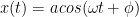


![x(t) = a(t) cos \left[ \phi (t) \right]](https://s0.wp.com/latex.php?latex=x%28t%29+%3D+a%28t%29+cos+%5Cleft%5B+%5Cphi+%28t%29+%5Cright%5D+&bg=ffffff&fg=000&s=0&c=20201002)


![z(t) = z_r(t) + j z_i(t) = x(t) + j HT \left[ x(t) \right]](https://s0.wp.com/latex.php?latex=z%28t%29+%3D+z_r%28t%29+%2B+j+z_i%28t%29+%3D+x%28t%29+%2B+j+HT+%5Cleft%5B+x%28t%29+%5Cright%5D+&bg=ffffff&fg=000&s=2&c=20201002)


![\phi(t) = \angle z(t) = arctan \left[ \frac{z_i(t)}{z_r(t)} \right]](https://s0.wp.com/latex.php?latex=%5Cphi%28t%29+%3D+%5Cangle+z%28t%29+%3D+arctan+%5Cleft%5B+%5Cfrac%7Bz_i%28t%29%7D%7Bz_r%28t%29%7D+%5Cright%5D+&bg=ffffff&fg=000&s=2&c=20201002)

![cos[\phi(t)]](https://s0.wp.com/latex.php?latex=cos%5B%5Cphi%28t%29%5D&bg=ffffff&fg=000&s=0&c=20201002)

