Numerous texts are available to explain the basics of Discrete Fourier Transform and its very efficient implementation – Fast Fourier Transform (FFT). Often we are confronted with the need to generate simple, standard signals (sine, cosine, Gaussian pulse, square wave, isolated rectangular pulse, exponential decay, chirp signal) for simulation purpose. I intend to show (in a series of articles) how these basic signals can be generated in Matlab and how to represent them in frequency domain using FFT.
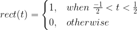
An isolated rectangular pulse of amplitude A and duration T is represented mathematically as
where
The Fourier transform of isolated rectangular pulse g(t) is
where, the sinc function is given by
Thus, the Fourier Transform pairs are
The Fourier Transform describes the spectral content of the signal at various frequencies. For a given signal g(t), the Fourier Transform is given by
where, the absolute value gives the magnitude of the frequency components (amplitude spectrum) and are their corresponding phase (phase spectrum) . For the rectangular pulse, the amplitude spectrum is given as
The amplitude spectrum peaks at f=0 with value equal to AT. The nulls of the spectrum occur at integral multiples of 1/T, i.e, ( )
Generating an isolated rectangular pulse in Matlab:
An isolated rectangular pulse of unit amplitude and width w (the factor T in equations above ) can be generated easily with the help of in-built function – rectpuls(t,w) command in Matlab. As an example, a unit amplitude rectangular pulse of duration is generated.
fs=500; %sampling frequency
T=0.2; %width of the rectangule pulse in seconds

t=-0.5:1/fs:0.5; %time base

x=rectpuls(t,T); %generating the square wave

plot(t,x,'k');
title(['Rectangular Pulse width=', num2str(T),'s']);
xlabel('Time(s)');
ylabel('Amplitude');
Amplitude spectrum using FFT:
Matlab’s FFT function is utilized for computing the Discrete Fourier Transform (DFT). The magnitude of FFT is plotted. From the following plot, it can be noted that the amplitude of the peak occurs at f=0 with peak value . The nulls in the spectrum are located at ().
L=length(x);
NFFT = 1024;
X = fftshift(fft(x,NFFT)); %FFT with FFTshift for both negative & positive frequencies
f = fs*(-NFFT/2:NFFT/2-1)/NFFT; %Frequency Vector

figure;
plot(f,abs(X)/(L),'r');
title('Magnitude of FFT');
xlabel('Frequency (Hz)')
ylabel('Magnitude |X(f)|');
Power spectral density (PSD) using FFT:
The distribution of power among various frequency components is plotted next. The first plot shows the double-side Power Spectral Density which includes both positive and negative frequency axis. The second plot describes the PSD only for positive frequency axis (as the response is just the mirror image of negative frequency axis).
figure;
Pxx=X.*conj(X)/(L*L); %computing power with proper scaling
plot(f,10*log10(Pxx),'r');
title('Double Sided - Power Spectral Density');
xlabel('Frequency (Hz)')
ylabel('Power Spectral Density- P_{xx} dB/Hz');
X = fft(x,NFFT);
X = X(1:NFFT/2+1);%Throw the samples after NFFT/2 for single sided plot
Pxx=X.*conj(X)/(L*L);
f = fs*(0:NFFT/2)/NFFT; %Frequency Vector
plot(f,10*log10(Pxx),'r');
title('Single Sided - Power Spectral Density');
xlabel('Frequency (Hz)')
ylabel('Power Spectral Density- P_{xx} dB/Hz');
Magnitude and phase spectrum:
The phase spectrum of the rectangular pulse manifests as series of pulse trains bounded between 0 and , provided the rectangular pulse is symmetrically centered around sample zero. This is explained in the reference here and the demo below.
clearvars;
x = [ones(1,7) zeros(1,127-13) ones(1,6)];
subplot(3,1,1); plot(x,'k');
title('Rectangular Pulse'); xlabel('Sample#'); ylabel('Amplitude');

NFFT = 127;
X = fftshift(fft(x,NFFT)); %FFT with FFTshift for both negative & positive frequencies
f = (-NFFT/2:NFFT/2-1)/NFFT; %Frequency Vector

subplot(3,1,2); plot(f,abs(X),'r');
title('Magnitude Spectrum'); xlabel('Frequency (Hz)'); ylabel('|X(f)|');

subplot(3,1,3); plot(f,atan2(imag(X),real(X)),'r');
title('Phase Spectrum'); xlabel('Frequency (Hz)'); ylabel('\angle X(f)');
Note: There is a rating embedded within this post, please visit this post to rate it.
Numerous texts are available to explain the basics of Discrete Fourier Transform and its very efficient implementation – Fast Fourier Transform (FFT). Often we are confronted with the need to generate simple, standard signals (sine, cosine, Gaussian pulse, squarewave, isolated rectangular pulse, exponential decay, chirp signal) for simulation purpose. I intend to show (in a series of articles) how these basic signals can be generated in Matlab and how to represent them in frequency domain using FFT.
The most logical way of transmitting information across a communication channel is through a stream of square pulse – a distinct pulse for ‘0‘ and another for ‘1‘. Digital signals are graphically represented as square waves with certain symbol/bit period. Square waves are also used universally in switching circuits, as clock signals synchronizing various blocks of digital circuits, as reference clock for a given system domain and so on.
Square wave manifests itself as a wide range of harmonics in frequency domain and therefore can cause electromagnetic interference. Square waves are periodic and contain odd harmonics when expanded as Fourier Series (where as signals like saw-tooth and other real word signals contain harmonics at all integer frequencies). Since a square wave literally expands to infinite number of odd harmonic terms in frequency domain, approximation of square wave is another area of interest. The number of terms of its Fourier Series expansion, taken for approximating the square wave is often seen as Gibbs Phenomenon, which manifests as ringing effect at the corners of the square wave in time domain (visual explanation here).
True Square waves are a special class of rectangular waves with 50% duty cycle. Varying the duty cycle of a rectangular wave leads to pulse width modulation, where the information is conveyed by changing the duty-cycle of each transmitted rectangular wave.
How to generate a square wave in Matlab
If you know the trick of generating a sine wave in Matlab, the task is pretty much simple. Square wave is generated using “square” function in Matlab. The command sytax – square(t,dutyCycle) – generates a square wave with period for the given time base. The command behaves similar to “sin” command (used for generating sine waves), but in this case it generates a square wave instead of a sine wave. The argument – dutyCycle is optional and it defines the desired duty cycle of the square wave. By default (when the dutyCycle argument is not supplied) the square wave is generated with (50%) duty cycle.
f=10; %frequency of sine wave in Hz
overSampRate=30; %oversampling rate
fs=overSampRate*f; %sampling frequency
duty_cycle=50; % Square wave with 50% Duty cycle (default)
nCyl = 5; %to generate five cycles of sine wave

t=0:1/fs:nCyl*1/f; %time base

x=square(2*pi*f*t,duty_cycle); %generating the square wave

plot(t,x,'k');
title(['Square Wave f=', num2str(f), 'Hz']);
xlabel('Time(s)');
ylabel('Amplitude');
Power Spectral Density using FFT
Let’s check out how the generated square wave will look in frequency domain. The Fast Fourier Transform (FFT) is utilized here. As discussed in the article here, there are numerous ways to plot the response of FFT. Single Sided power spectral density is plotted first, followed by the Double-sided power spectral density.
Single Sided Power Spectral Density
X = fft(x,NFFT);
X = X(1:NFFT/2+1);%Throw the samples after NFFT/2 for single sided plot
Pxx=X.*conj(X)/(NFFT*L);
f = fs*(0:NFFT/2)/NFFT; %Frequency Vector

plot(f,10*log10(Pxx),'r');
title('Single Sided Power Spectral Density');
xlabel('Frequency (Hz)')
ylabel('Power Spectral Density- P_{xx} dB/Hz');
ylim([-45 -5])
Double Sided Power Spectral Density
L=length(x);
NFFT = 1024;
X = fftshift(fft(x,NFFT));
Pxx=X.*conj(X)/(NFFT*L); %computing power with proper scaling
f = fs*(-NFFT/2:NFFT/2-1)/NFFT; %Frequency Vector

plot(f,10*log10(Pxx),'r');
title('Double Sided Power Spectral Density');
xlabel('Frequency (Hz)')
ylabel('Power Spectral Density- P_{xx} dB/Hz');
Note: There is a rating embedded within this post, please visit this post to rate it.
Key focus: Learn how to plot FFT of sine wave and cosine wave using Matlab. Understand FFTshift. Plot one-sided, double-sided and normalized spectrum.
Introduction
Numerous texts are available to explain the basics of Discrete Fourier Transform and its very efficient implementation – Fast Fourier Transform (FFT). Often we are confronted with the need to generate simple, standard signals (sine, cosine, Gaussian pulse, squarewave, isolated rectangular pulse, exponential decay, chirp signal) for simulation purpose. I intend to show (in a series of articles) how these basic signals can be generated in Matlab and how to represent them in frequency domain using FFT. If you are inclined towards Python programming, visit here.
In order to generate a sine wave in Matlab, the first step is to fix the frequency of the sine wave. For example, I intend to generate a f=10 Hz sine wave whose minimum and maximum amplitudes are and respectively. Now that you have determined the frequency of the sinewave, the next step is to determine the sampling rate. Matlab is a software that processes everything in digital. In order to generate/plot a smooth sine wave, the sampling rate must be far higher than the prescribed minimum required sampling rate which is at least twice the frequency – as per Nyquist Shannon Theorem. A oversampling factor of is chosen here – this is to plot a smooth continuous-like sine wave (If this is not the requirement, reduce the oversampling factor to desired level). Thus the sampling rate becomes . If a phase shift is desired for the sine wave, specify it too.
f=10; %frequency of sine wave
overSampRate=30; %oversampling rate
fs=overSampRate*f; %sampling frequency
phase = 1/3*pi; %desired phase shift in radians
nCyl = 5; %to generate five cycles of sine wave

t=0:1/fs:nCyl*1/f; %time base

x=sin(2*pi*f*t+phase); %replace with cos if a cosine wave is desired
plot(t,x);
title(['Sine Wave f=', num2str(f), 'Hz']);
xlabel('Time(s)');
ylabel('Amplitude');
Representing in Frequency Domain
Representing the given signal in frequency domain is done via Fast Fourier Transform (FFT) which implements Discrete Fourier Transform (DFT) in an efficient manner. Usually, power spectrum is desired for analysis in frequency domain. In a power spectrum, power of each frequency component of the given signal is plotted against their respective frequency. The command computes the -point DFT. The number of points – – in the DFT computation is taken as power of (2) for facilitating efficient computation with FFT. A value of is chosen here. It can also be chosen as next power of 2 of the length of the signal.
Different representations of FFT:
Since FFT is just a numeric computation of -point DFT, there are many ways to plot the result.
1. Plotting raw values of DFT:
The x-axis runs from to – representing sample values. Since the DFT values are complex, the magnitude of the DFT is plotted on the y-axis. From this plot we cannot identify the frequency of the sinusoid that was generated.
2. FFT plot – plotting raw values against Normalized Frequency axis:
In the next version of plot, the frequency axis (x-axis) is normalized to unity. Just divide the sample index on the x-axis by the length of the FFT. This normalizes the x-axis with respect to the sampling rate . Still, we cannot figure out the frequency of the sinusoid from the plot.
3. FFT plot – plotting raw values against normalized frequency (positive & negative frequencies):
As you know, in the frequency domain, the values take up both positive and negative frequency axis. In order to plot the DFT values on a frequency axis with both positive and negative values, the DFT value at sample index has to be centered at the middle of the array. This is done by using function in Matlab. The x-axis runs from to where the end points are the normalized ‘folding frequencies’ with respect to the sampling rate .
4. FFT plot – Absolute frequency on the x-axis Vs Magnitude on Y-axis:
Here, the normalized frequency axis is just multiplied by the sampling rate. From the plot below we can ascertain that the absolute value of FFT peaks at and . Thus the frequency of the generated sinusoid is . The small side-lobes next to the peak values at and are due to spectral leakage.
5. Power Spectrum – Absolute frequency on the x-axis Vs Power on Y-axis:
The following is the most important representation of FFT. It plots the power of each frequency component on the y-axis and the frequency on the x-axis. The power can be plotted in linear scale or in log scale. The power of each frequency component is calculated as Where is the frequency domain representation of the signal . In Matlab, the power has to be calculated with proper scaling terms (since the length of the signal and transform length of FFT may differ from case to case).
NFFT=1024;
L=length(x);
X=fftshift(fft(x,NFFT));
Px=X.*conj(X)/(NFFT*L); %Power of each freq components
fVals=fs*(-NFFT/2:NFFT/2-1)/NFFT;
plot(fVals,Px,'b');
title('Power Spectral Density');
xlabel('Frequency (Hz)')
ylabel('Power');
NFFT=1024;
L=length(x);
X=fftshift(fft(x,NFFT));
Px=X.*conj(X)/(NFFT*L); %Power of each freq components
fVals=fs*(-NFFT/2:NFFT/2-1)/NFFT;
plot(fVals,10*log10(Px),'b');
title('Power Spectral Density');
xlabel('Frequency (Hz)')
ylabel('Power');
6. Power Spectrum – One-Sided frequencies
In this type of plot, the negative frequency part of x-axis is omitted. Only the FFT values corresponding to to sample points of -point DFT are plotted. Correspondingly, the normalized frequency axis runs between to . The absolute frequency (x-axis) runs from to .
L=length(x);
NFFT=1024;
X=fft(x,NFFT);
Px=X.*conj(X)/(NFFT*L); %Power of each freq components
fVals=fs*(0:NFFT/2-1)/NFFT;
plot(fVals,Px(1:NFFT/2),'b','LineSmoothing','on','LineWidth',1);
title('One Sided Power Spectral Density');
xlabel('Frequency (Hz)')
ylabel('PSD');
Rate this article: Note: There is a rating embedded within this post, please visit this post to rate it.
Correlation matrix defines correlation among N variables. It is a symmetric matrix with the element equal to the correlation coefficient between the and the variable. The diagonal elements (correlations of variables with themselves) are always equal to 1.
Sample problem:
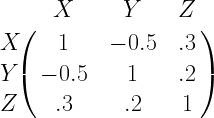
Let’s say we would like to generate three sets of random sequences X,Y,Z with the following correlation relationships.
Correlation co-efficient between X and Y is 0.5
Correlation co-efficient between X and Z is 0.3
Obviously the variable X correlates with itself 100% – i.e, correlation-coefficient is 1
Putting all these relationships in a compact matrix form, gives the correlation matrix. We take arbitrary correlation value (0.3) for the relationship between Y and Z.
Now, the task is to generate three sets of random numbers X,Y and Z that follows the relationship above. The problem can be addressed in many ways. Two most common methods finding the solution are
Generating Correlated random number using Cholesky Decomposition:
Cholesky decomposition is the matrix equivalent of taking square root operation on a given matrix. As with any scalar values, positive square root is only possible if the given number is a positive (Imaginary roots do exist otherwise). Similarly, if a matrix need to be decomposed into square-root equivalent, the matrix need to be positive definite.
The method discussed here, seeks to decompose the given correlation matrix using Cholesky decomposition.
where U and L are upper and lower triangular matrices. We will consider Upper triangular matrix here. Equivalently, lower triangular matrix can also be used, in which case the order of output needs to be reversed.
For this decomposition to work, the correlation matrix should be positive definite. The correlated random sequences (where X,Y,Z are column vectors) that follow the above relationship can be generated by multiplying the uncorrelated random numbers R with U .
Steps to follow:
Generate three sequences of uncorrelated random numbers R – each drawn from a normal distribution. For this case, the R matrix will be of size where k is the number of samples we wish to generate and we allocate the k samples in three columns, where the columns indicate the place holder for each variable X, Y and Z. Multiply this matrix with the Cholesky decomposed upper triangular version of the correlation matrix.
Python code
import numpy as np
from scipy.linalg import cholesky
from scipy.stats import pearsonr #to calculate correlation coefficient

#for plotting and visualization
import pandas as pd
import matplotlib.pyplot as plt
%matplotlib inline
plt.style.use('fivethirtyeight')
import seaborn as sns

C = np.array([[1, -0.5, 0.3],
              [-0.5, 1, 0.2],
              [0.3, 0.2, 1]]) #Construct correlation matrix
U = cholesky(C) #Cholesky decomposition
R = np.random.randn(10000,3) #Three uncorrelated sequences
Rc = R @ U #Array of correlated random sequences

#compute and display correlation coeff from generated sequences
def pearsonCorr(x, y, **kws):
    (r, _) = pearsonr(x, y) #returns Pearson’s correlation coefficient, 2-tailed p-value)
    ax = plt.gca()
    ax.annotate("r = {:.2f} ".format(r),xy=(.7, .9), xycoords=ax.transAxes)

#Visualization
df = pd.DataFrame(data=Rc, columns=['X','Y','Z'])
graph = sns.pairplot(df)
graph.map(pearsonCorr)
Figure 1: Pairplot of correlated random variables generated using Cholesky decomposition (Python)
Matlab code
x=[  1  0.5 0.3; 0.5  1  0.3; 0.3 0.3  1 ;]; %Correlation matrix
U=chol(x); %Cholesky decomposition

R=randn(10000,3); %Random data in three columns each for X,Y and Z
Rc=R*U; %Correlated matrix Rc=[X Y Z]

%Verify Correlation-Coeffs of generated vectors
coeffMatrixXX=corrcoef(Rc(:,1),Rc(:,1));
coeffMatrixXY=corrcoef(Rc(:,1),Rc(:,2));
coeffMatrixXZ=corrcoef(Rc(:,1),Rc(:,3));

%Extract the required correlation coefficients
coeffXX=coeffMatrixXX(1,2) %Correlation Coeff for XX;
coeffXY=coeffMatrixXY(1,2) %Correlation Coeff for XY;
coeffXZ=coeffMatrixXZ(1,2) %Correlation Coeff for XZ;

%Scatterplots
subplot(3,1,1)
plot(Rc(:,1),Rc(:,1),'b.')
title(['Scatterd Plot - X and X calculated \rho=' num2str(coeffXX)])
xlabel('X')
ylabel('X')

subplot(3,1,2)
plot(Rc(:,1),Rc(:,2),'r.')
title(['Scatterd Plot - X and Y calculated \rho=' num2str(coeffXY)])
xlabel('X')
ylabel('Y')

subplot(3,1,3)
plot(Rc(:,1),Rc(:,3),'m.')
title(['Scatterd Plot - X and Z calculated \rho=' num2str(coeffXZ)])
xlabel('X')
ylabel('Z')
Generating two vectors of correlated random numbers, given the correlation coefficient , is implemented in two steps. The first step is to generate two uncorrelated random sequences from an underlying distribution. Normally distributed random sequences are considered here.
Mathematical details of convolution, its relationship to polynomial multiplication and the application of Toeplitz matrices in computing linear convolution are discussed in the previous article. A short survey of different techniques to compute discrete linear convolution (with Matlab code) is given here.
Definition
Given an LTI (Linear Time Invariant) system with impulse response \(h[n]\) and an input sequence \(x[n]\), the output of the system \(y[n]\) is obtained by convolving the input sequence and impulse response.
The above equation can simply be implemented using nested for-loops, which consume the most computational time of all the methods given here. Typically, the computational complexity is \(O(n^2)\) time.
Python
def conv_brute_force(x,h):
	"""
	Brute force method to compute convolution
	Parameters:
	x, h : numpy vectors
	Returns:
		y : convolution of x and h
	"""
	N=len(x)
	M=len(h)
	y = np.zeros(N+M-1) #array filled with zeros

	for i in np.arange(0,N):
		for j in np.arange(0,M):
			y[i+j] = y[i+j] + x[i] * h[j]
return y
Matlab
for i = 0:n+m,
   yi = 0;
for i = 0 :n,
   for k = 0 to m,
      y[i+k] = y[i+k] + x[i] · h[k];
Method 2 – Using Toeplitz Matrix:
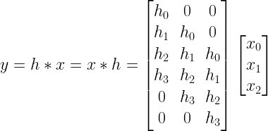
When the sequences \(h[n]\) and \(x[n]\) are represented as matrices, the linear convolution operation can be equivalently represented as
\[y=h \ast x=x \ast h=Toeplitz(h) X\]
Assume that the sequence \(h[n]\) is of length 4 given by \(h[n]=[h_0,h_1,h_2,h_3]\) and the sequence \(x[n]\) is of length 3 given by \(x[n]=[x_0,x_1,x_2]\). The convolution \(h[n] \ast x[n]\) is given by
The matrix representing the incremental delays of \(h[n]\) used in the above equation is a special form of matrix called Toeplitz matrix. Toeplitz matrix have constant entries along their diagonals. Toeplitz matrices are used to model systems that posses shift invariant properties. The property of shift invariance is evident from the matrix structure itself. Since we are modelling a Linear Time Invariant system[1], Toeplitz matrices are our natural choice. On a side note, a special form of Toeplitz matrix called “circulant matrix” is used in applications involving circular convolution and Discrete Fourier Transform (DFT)[2].
In Matlab, it is constructed by calling Toeplitz function[3] with two arguments. The first argument is the first column of the above matrix -\( [h_0,h_1,h_2,h_3,0,0]\) and the second argument is the first row of the above matrix – \([h_0,0,0]\).
y=toeplitz([h0 h1 h2 h3 0 0],[h0 0 0])*x.';
In the generalized case, where \(x\) and \(h\) are of any arbitrary lengths (say \(N\) and \(M\)), the code can be modified as follows [here it is assumed that \( length (x) \geq length(h)\) ]
Computation of convolution using FFT (Fast Fourier Transform) has the advantage of reduced computational complexity when the length of inputs are large. To compute convolution, take FFT of the two sequences \(x\) and \(h\) with FFT length set to convolution output length \(length (x)+length(h)-1\), multiply the results and convert back to time-domain using IFFT (Inverse Fast Fourier Transform). Note that FFT is a direct implementation of circular convolution in time domain. Here we are attempting to compute linear convolution using circular convolution (or FFT) with zero-padding either one of the input sequence. This causes inefficiency when compared to circular convolution. Nevertheless, this method still provides \(O\left(\frac{N}{log_2N}\right)\) savings over brute-force method.
from scipy.fftpack import fft,ifft
y=ifft(fft(x,L)*(fft(h,L))) #Convolution using FFT and IFFT
Matlab
y=ifft(fft(x,L).*(fft(h,L)))
Other Methods:
If the input sequence is of infinite length or very very large as in many real time applications, block processing methods like Overlap-Add and Overlap-Save methods can be used to compute convolution in a faster and efficient way.
Standard Algorithms for Fast Convolution:
Standard algorithms for computing convolution that greatly reduce the computational complexity are
Refer [4] -Fast Algorithms for Signal Processing by Richard E. Blahut for more details on the above algorithms (see reference section below).
Matlab Code
Implementing method 2 (convolution using Toeplitz matrix transformation) and method 3 (convolution using FFT) and comparing against Matlab’s standard conv function:
%Create random vectors for test
x=rand(1,7)+1i*rand(1,7);
h=rand(1,3)+1i*rand(1,3);
L=length(x)+length(h)-1;

%Convolution Using Toeplitz matrix
y1=toeplitz([h zeros(1,length(x)-1)],[h(1) zeros(1,length(x)-1)])*x.'
%Convolution FFT
y2=ifft(fft(x,L).*(fft(h,L))).'
%Matlab's standard function
y3=conv(h,x).'
Simulation output:
Comparing method 2 and method 3 against Matlab’s standard convolution function returns identical results
Convolution operation is ubiquitous in signal processing applications. The mathematics of convolution is strongly rooted in operation on polynomials. The intent of this text is to enhance the understanding on mathematical details of convolution.
Polynomial functions:
Polynomial functions are expressions consisting of sum of terms, where each term includes one or more variables raised to a non-negative power and each term may be scaled by a coefficient. Addition, Subtraction and multiplication of polynomials are possible.
Polynomial functions can involve one or more variables. For example, following polynomial expression is a function of variable x. It involves sum of 3 terms where each term is scaled by a coefficient. Polynomial expression involving two variables ‘x’ and ‘y’ is given next.
Representing single variable polynomial functions:
Polynomial functions involving single variable is of specific interest here. In general a single variable (say ‘x’) polynomial is expressed in the following sum of terms form, where are coefficients of the polynomial.
The degree or order of the polynomial function is the highest power of with a non-zero coefficient. The above equation can be written as
It is also represented by a vector of coefficients as .
Polynomials can also be represented using their roots which is a product of linear terms form, as explained later.
Multiplication of polynomials and linear convolution:
As indicated earlier, mathematical operations like additions, subtractions and multiplications can be performed on polynomial functions. Addition or subtraction of polynomials is straight forward. Multiplication of polynomials is of specific interest in the context of subject discussed here.
Computing the product of two polynomials represented by the coefficient vectors and . The usual representation of such polynomials is given by
The product vector is represented as
Or equivalently as
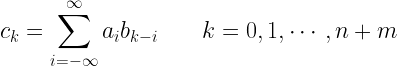
Since the subscripts obey the equality , changing the subscript to gives
Which, when written in terms of indices, provides the most widely used form seen in signal processing text books.
This operation is referred as convolution (linear convolution, to be precise), denoted as . It is very closely related to other operations on vectors – cross-correlation, auto-correlation and moving average computation. Thus when we are computing convolution, we are actually multiplying two polynomials.
Note, that if the polynomials have and terms, their multiplication produces terms.
The straightforward algorithm (shown below) that implements the above product expression will consume time. A better algorithm is a necessity. It turns out that viewing the polynomials as product of linear factors of complex roots will save much of the computations. This forms the basis for Fast Fourier Transform, where nth root of unity is utilized recursively to do the computation in frequency domain (in signal processing perspective). More about this later.
for i = 0:n+m,
   ci = 0;
for i = 0 :n,
   for k = 0 to m,
      c[i+k] = c[i+k] + a[i] · b[k];
Toeplitz Matrix and Convolution:
Convolution operation of two sequences can be viewed as multiplying two matrices as explained next. Given a LTI (Linear Time Invariant) system with impulse response and an input sequence , the output of the system is obtained by convolving the input sequence and impulse response.
where, the sequence is of length and is of length .
Assume that the sequence is of length 4 given by and the sequence is of length 3 given by . The convolution is given by
Computing each sample in the convolution,
Note the above result. See how the series and multiply with each other from the opposite directions. This gives the reason on why we have to reverse one of the sequences and shift one step a time to do the convolution operation (This is often depicted graphically on standard signal processing texts.. You might have wondered why we have to do this… Now, rejoice that you have understood the reason behind it)
Thus, graphically, in convolution, one of the sequences (say ) is reversed. It is delayed to the extreme left where there are no overlaps between the two sequences. Now, the sample offset of is increased 1 step at a time. At each step, the overlapping portions of and are multiplied and summed. This process is repeated till the sequence is slid to the extreme right where no more overlaps between and are possible.
Writing the final result in the previous equation in matrix form,
When the sequences and are represented as matrices, the convolution operation can be equivalently represented as
The matrix representing the incremental delays of used in the above equation is a special form of matrix called Toeplitz matrix. Toeplitz matrix have constant entries along their diagonals. Toeplitz matrices are used to model systems that posses shift invariant properties. The property of shift invariance is evident from the matrix structure itself. Since we are modelling a Linear Time Invariant system[1], Toeplitz matrices are our natural choice. On a side note, a special form of Toeplitz matrix called “circulant matrix” is used in applications involving circular convolution and Discrete Fourier Transform (DFT)[2].
Representing the operation used to construct the Toeplitz matrix out of the sequence as ,
Now, the convolution of and is simply a matrix multiplication of Toeplitz matrix and the matrix representation of denoted as
One can quickly vectorize the convolution operation in matlab by using Toeplize matrices as shown below.
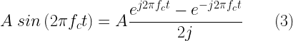
Let x(t) be a sine wave of amplitude A and frequency fc represented by the following equation.
When represented in frequency domain, it will look like the one on the right side plot in the following figure. This is evident from the fact that the sinewave can be mathematically represented by applying Euler’s formula.
Taking the Fourier transform of x(t) to represent it in frequency domain,
When considering the amplitude part,the above decomposition gives two spikes of amplitude A/2 on either side of the frequency domain at fc and -fc.
Figure 1: Time domain representation and frequency spectrum of a pure sinewave
Squaring the amplitudes gives the magnitude of power of the individual spikes/frequency components. The power spectrum is plotted below.
Figure 2: Power spectrum of a pure sinewave
Thus if the pure sinewave is of amplitude A=1V and frequency=100Hz, the power spectrum will have two spikes of value at 100 Hz and -100 Hz frequencies. The total power will be
Let’s verify this through simulation.
Simulation and Verification
A sine wave of 100 Hz frequency and amplitude 1V is taken for the experiment.
A=1; %Amplitude of sine wave
Fc=100; %Frequency of sine wave
Fs=1000; %Sampling rate - oversampled by the rate of 10
Ts=1/Fs; %Sampling period
nCycles=200; %Number of cycles of the sinewave

subplot(2,1,1);
t=0:Ts:nCycles/Fc-Ts; %Time base
x=A*sin(2*pi*Fc*t); %Sinusoidal function
stem(t,x); %Plot command
A sinusoidal wave of 10 cycles is plotted here
Figure 3: Sine wave generated in Matlab
Matlab’s Norm function:
Matlab’s basic installation comes with “norm” function. The p-norm in Matlab is computed as
By default, the single argument norm function computed 2-norm given as
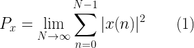
To compute the total power of the signal x[n] (as in equation (1) above), all we have to do is – compute norm(x), square it and divide by the length of the signal.
L=length(x);
P=(norm(x)^2)/L;
sprintf('Power of the Signal from Time domain %f',P);
The above given piece of code will result in the following output
Power of the Signal from Time domain 0.500000
Verifying the total Power by DFT : Frequency Domain
Here, the total power is verified by applying DFT on the sinusoidal sequence. The sinusoidal sequence x[n] is represented in frequency domain X[f] using Matlab’s FFT function. The power associated with each frequency point is computed as
Finally, the total power is calculated as the sum of all the points in the frequency domain representation.
X = fft(x);
Px=sum(X.*conj(X))/(L^2); %Compute power with proper scaling.
subplot(2,1,2)
% Plot single-sided amplitude spectrum.
stem(Px);
sprintf('Total Power of the Signal from DFT %f',P);
Result:
Total Power of the Signal from DFT 0.500000
Figure 4: Power spectrum of a pure sinewave simulated in Matlab
A word on Matlab’s FFT: Matlab’s FFT is optimized for faster performance if the transform length is a power of 2. The following snippet of code simply calls “fft” without the transform length. In this case, the window length and the transform length are the same. This is to simplify the calculation of power. You can re-write the call to the FFT routine with transform length set to next power of two which is greater than or equal to the window length (sequence length). Then the step to compute total power will be differing slightly in the denominator. But that will not improve resolution (Remember : zero padding to compute FFT will not improve resolution).
Also note that in the above simulation we are using a pure sinusoid. The entire sequence of sinusoid defined all the cycles completely. There are no discontinuities in the sequence. If you call FFT with the transform length set to next power of 2 (as given in Matlab manuals), it will pad additional zeros to the sequence and creates discontinuities in the FFT computation. This will lead to spectral leakage. FFT and spectral leakage is discussed here.
Rate this article: Note: There is a rating embedded within this post, please visit this post to rate it.
Key focus: Clearly understand the terms: power and energy of a signal, their mathematical definition, physical significance and computation in signal processing context.
Energy of a signal:
Defining the term “size”:
In signal processing, a signal is viewed as a function of time. The term “size of a signal” is used to represent “strength of the signal”. It is crucial to know the “size” of a signal used in a certain application. For example, we may be interested to know the amount of electricity needed to power a LCD monitor as opposed to a CRT monitor. Both of these applications are different and have different tolerances. Thus the amount of electricity driving these devices will also be different.
A given signal’s size can be measured in many ways. Given a mathematical function (or a signal equivalently), it seems that the area under the curve, described by the mathematical function, is a good measure of describing the size of a signal. A signal can have both positive and negative values. This may render areas that are negative. Due to this effect, it is possible that the computed values cancel each other totally or partially, rendering incorrect result. Thus the metric function of “area under the curve” is not suitable for defining the “size” of a signal. Now, we are left with two options : either 1) computation of the area under the absolute value of the function or 2) computation of the area under the square of the function. The second choice is favored due to its mathematical tractability and its similarity to Euclidean Norm which is used in signal detection techniques (Note: Euclidean norm – otherwise called L2 norm or 2-norm[1] – is often considered in signal detection techniques – on the assumption that it provides a reasonable measure of distance between two points on signal space. It is computed as Euclidean distance in detection theory).
Going by the second choice of viewing the “size” as the computation of the area under the square of the function, the energy of a continuous-time complex signal \(x(t)\) is defined as
\[E_x = \int_{-\infty}^{\infty} |x(t)|^2 dt\]
If the signal \(x(t)\) is real, the modulus operator in the above equation does not matter.
This is called “Energy” in signal processing terms. This is also a measure of signal strength. This definition can be applied to any signal (or a vector) irrespective of whether it possesses actual energy (a basic quantitative property as described by physics) or not. If the signal is associated with some physical energy, then the above definition gives the energy content in the signal. If the signal is an electrical signal, then the above definition gives the total energy of the signal (in Joules) dissipated over a 1 Ohm resistor.
Actual Energy – physical quantity:
To know the actual energy of the signal \(E\), one has to know the value of load \(Z\) the signal is driving and also the nature the electrical signal (voltage or current). For a voltage signal, the above equation has to be scaled by a factor of \(1/Z\).
\[E = ZE_x = Z \int_{-\infty}^{\infty} |x(t)|^2 dt\]
Here, \(Z\) is the impedance driven by the signal \(x(t)\) , \(E_x\) is the signal energy (signal processing term) and \(E\) is the Energy of the signal (physical quantity) driving the load \( Z\)
Energy in discrete domain:
In the discrete domain, the energy of the signal is given by
The energy is finite only if the above sum converges to a finite value. This implies that the signal is “squarely-summable“. Such a signal is called finite energy signal.
What if the given signal does not decay with respect to time (as in a continuous sine wave repeating its cycle infinitely) ? The energy will be infinite and such a signal is “not squarely-summable” in other words. We need another measurable quantity to circumvent this problem.This leads us to the notion of “Power”
Power:
Power is defined as the amount of energy consumed per unit time. This quantity is useful if the energy of the signal goes to infinity or the signal is “not-squarely-summable”. For “non-squarely-summable” signals, the power calculated by taking the snapshot of the signal over a specific interval of time as follows
1) Take a snapshot of the signal over some finite time duration 2) Compute the energy of the signal \(E_x\) 3) Divide the energy by number of samples taken for computation \(N\) 4) Extend the limit of number of samples to infinity \(N\rightarrow \infty \). This gives the total power of the signal.
In discrete domain, the total power of the signal is given by
Following equations are different forms of the same computation found in many text books. The only difference is the number of samples taken for computation. The denominator changes according to the number of samples taken for computation.
A signal can be classified based on its power or energy content. Signals having finite energy are energy signals. Power signals have finite and non-zero power.
Energy Signal :
A finite energy signal will have zero TOTAL power. Let’s investigate this statement in detail. When the energy is finite, the total power will be zero. Check out the denominator in the equation for calculating the total power. When the limit \(N\rightarrow \infty\), the energy dilutes to zero over the infinite duration and hence the total power becomes zero.
Power Signal:
Signals whose total power is finite and non-zero. The energy of the power signal will be infinite. Example: Periodic sequences like sinusoid. A sinusoidal signal has finite, non-zero power but infinite energy.
A signal cannot be both an energy signal and a power signal.
Neither an Energy signal nor a Power signal:
Signals can also be a cat on the wall – neither an energy signal nor a power signal. Consider a signal of increasing amplitude defined by,
\[x(n) = n\]
For such a signal, both the energy and power will be infinite. Thus, it cannot be classified either as an energy signal or as a power signal.
A random process (or signal for your visualization) with a constant power spectral density (PSD) function is a white noise process.
Power Spectral Density
Power Spectral Density function (PSD) shows how much power is contained in each of the spectral component. For example, for a sine wave of fixed frequency, the PSD plot will contain only one spectral component present at the given frequency. PSD is an even function and so the frequency components will be mirrored across the Y-axis when plotted. Thus for a sine wave of fixed frequency, the double sided plot of PSD will have two components – one at +ve frequency and another at –ve frequency of the sine wave. (Know how to plot PSD/FFT in Python & in Matlab)
Gaussian and Uniform White Noise:
A white noise signal (process) is constituted by a set of independent and identically distributed (i.i.d) random variables. In discrete sense, the white noise signal constitutes a series of samples that are independent and generated from the same probability distribution. For example, you can generate a white noise signal using a random number generator in which all the samples follow a given Gaussian distribution. This is called White Gaussian Noise (WGN) or Gaussian White Noise. Similarly, a white noise signal generated from a Uniform distribution is called Uniform White Noise.
Gaussian Noise and Uniform Noise are frequently used in system modelling. In modelling/simulation, white noise can be generated using an appropriate random generator. White Gaussian Noise can be generated using randn function in Matlab which generates random numbers that follow a Gaussian distribution. Similarly, rand function can be used to generate Uniform White Noise in Matlab that follows a uniform distribution. When the random number generators are used, it generates a series of random numbers from the given distribution. Let’s take the example of generating a White Gaussian Noise of length 10 using randn function in Matlab – with zero mean and standard deviation=1.
This simply generates 10 random numbers from the standard normal distribution. As we know that a white process is seen as a random process composing several random variables following the same Probability Distribution Function (PDF). The 10 random numbers above are generated from the same PDF (standard normal distribution). This condition is called “identically distributed” condition. The individual samples given above are “independent” of each other. Furthermore, each sample can be viewed as a realization of one random variable. In effect, we have generated a random process that is composed of realizations of 10 random variables. Thus, the process above is constituted from “independent identically distributed” (i.i.d) random variables.
Strictly and weakly defined white noise:
Since the white noise process is constructed from i.i.d random variable/samples, all the samples follow the same underlying probability distribution function (PDF). Thus, the Joint Probability Distribution function of the process will not change with any shift in time. This is called a stationary process. Hence, this noise is a stationary process. As with a stationary process which can be classified as Strict Sense Stationary (SSS) and Wide Sense Stationary (WSS) processes, we can have white noise that is SSS and white noise that is WSS. Correspondingly they can be called strictly defined white noise signal and weakly defined white noise signal.
What’s with Covariance Function/Matrix ?
A white noise signal, denoted by \(x(t)\), is defined in weak sense is a more practical condition. Here, the samples are statistically uncorrelated and identically distributed with some variance equal to \(\sigma^2\). This condition is specified by using a covariance function as
\[COV \left(x_i, x_j \right) = \begin{cases} \sigma^2, & \quad i = j \\ 0, & \quad i \neq j \end{cases}\]
Why do we need a covariance function? Because, we are dealing with a random process that is composed of \(n\) random variables (10 variables in the modelling example above). Such a process is viewed as multivariate random vector or multivariate random variable.
For multivariate random variables, Covariance function specified how each of the \(n\) variables in the given random process behaves with respect to each other. Covariance function generalizes the notion of variance to multiple dimensions.
The above equation when represented in the matrix form gives the covariance matrix of the white noise random process. Since the random variables in this process are statistically uncorrelated, the covariance function contains values only along the diagonal.
The matrix above indicates that only the auto-correlation function exists for each random variable. The cross-correlation values are zero (samples/variables are statistically uncorrelated with respect to each other). The diagonal elements are equal to the variance and all other elements in the matrix are zero.The ensemble auto-correlation function of the weakly defined white noise is given by This indicates that the auto-correlation function of weakly defined white noise process is zero everywhere except at lag \(\tau=0\).
\[R_{xx}(\tau) = E \left[ x(t) x^*(t-\tau)\right] = \sigma^2 \delta (\tau)\]
Wiener-Khintchine Theorem states that for Wide Sense Stationary Process (WSS), the power spectral density function \(S_{xx}(f)\) of a random process can be obtained by Fourier Transform of auto-correlation function of the random process. In continuous time domain, this is represented as
\[S_{xx}(f) = F \left[R_{xx}(\tau) \right] = \int_{-\infty}^{\infty} R_{xx} (\tau) e ^{- j 2 \pi f \tau} d \tau\]
For the weakly defined white noise process, we find that the mean is a constant and its covariance does not vary with respect to time. This is a sufficient condition for a WSS process. Thus we can apply Weiner-Khintchine Theorem. Therefore, the power spectral density of the weakly defined white noise process is constant (flat) across the entire frequency spectrum (Figure 1). The value of the constant is equal to the variance or power of the noise signal.
\[S_{xx}(f) = F \left[R_{xx}(\tau) \right] = \int_{-\infty}^{\infty} \sigma^2 \delta (\tau) e ^{- j 2 \pi f \tau} d \tau = \sigma^2 \int_{-\infty}^{\infty} \delta (\tau) e ^{- j 2 \pi f \tau} = \sigma^2\]
Figure 1: Weiner-Khintchine theorem illustrated
Testing the characteristics of White Gaussian Noise in Matlab:
Generate a Gaussian white noise signal of length \(L=100,000\) using the randn function in Matlab and plot it. Let’s assume that the pdf is a Gaussian pdf with mean \(\mu=0\) and standard deviation \(\sigma=2\). Thus the variance of the Gaussian pdf is \(\sigma^2=4\). The theoretical PDF of Gaussian random variable is given by
subplot(2,1,2)
n=100; %number of Histrogram bins
[f,x]=hist(X,n);
bar(x,f/trapz(x,f)); hold on;
%Theoretical PDF of Gaussian Random Variable
g=(1/(sqrt(2*pi)*sigma))*exp(-((x-mu).^2)/(2*sigma^2));
plot(x,g);hold off; grid on;
title('Theoretical PDF and Simulated Histogram of White Gaussian Noise');
legend('Histogram','Theoretical PDF');
xlabel('Bins');
ylabel('PDF f_x(x)');
Figure 3: Plot of simulated & theoretical PDF for Gaussian RV
Compute the auto-correlation function of the white noise. The computed auto-correlation function has to be scaled properly. If the ‘xcorr’ function (inbuilt in Matlab) is used for computing the auto-correlation function, use the ‘biased’ argument in the function to scale it properly.
figure();
Rxx=1/L*conv(flipud(X),X);
lags=(-L+1):1:(L-1);

%Alternative method
%[Rxx,lags] =xcorr(X,'biased');
%The argument 'biased' is used for proper scaling by 1/L
%Normalize auto-correlation with sample length for proper scaling

plot(lags,Rxx);
title('Auto-correlation Function of white noise');
xlabel('Lags')
ylabel('Correlation')
grid on;
Figure 4: Autocorrelation function of generated noise
Simulating the PSD:
Simulating the Power Spectral Density (PSD) of the white noise is a little tricky business. There are two issues here 1) The generated samples are of finite length. This is synonymous to applying truncating an infinite series of random samples. This implies that the lags are defined over a fixed range. ( FFT and spectral leakage – an additional resource on this topic can be found here) 2) The random number generators used in simulations are pseudo-random generators. Due these two reasons, you will not get a flat spectrum of psd when you apply Fourier Transform over the generated auto-correlation values.The wavering effect of the psd can be minimized by generating sufficiently long random signal and averaging the psd over several realizations of the random signal.
Simulating Gaussian White Noise as a Multivariate Gaussian Random Vector:
To verify the power spectral density of the white noise, we will use the approach of envisaging the noise as a composite of \(N\) Gaussian random variables. We want to average the PSD over \(L\) such realizations. Since there are \(N\) Gaussian random variables (\(N\) individual samples) per realization, the covariance matrix \( C_{xx}\) will be of dimension \(N \times N\). The vector of mean for this multivariate case will be of dimension \(1 \times N\).
Cholesky decomposition of covariance matrix gives the equivalent standard deviation for the multivariate case. Cholesky decomposition can be viewed as square root operation. Matlab’s randn function is used here to generate the multi-dimensional Gaussian random process with the given mean matrix and covariance matrix.
%Verifying the constant PSD of White Gaussian Noise Process
%with arbitrary mean and standard deviation sigma

mu=0; %Mean of each realization of Noise Process
sigma=2; %Sigma of each realization of Noise Process

L = 1000; %Number of Random Signal realizations to average
N = 1024; %Sample length for each realization set as power of 2 for FFT

%Generating the Random Process - White Gaussian Noise process
MU=mu*ones(1,N); %Vector of mean for all realizations
Cxx=(sigma^2)*diag(ones(N,1)); %Covariance Matrix for the Random Process
R = chol(Cxx); %Cholesky of Covariance Matrix
%Generating a Multivariate Gaussian Distribution with given mean vector and
%Covariance Matrix Cxx
z = repmat(MU,L,1) + randn(L,N)*R;
Compute PSD of the above generated multi-dimensional process and average it to get a smooth plot.
%By default, FFT is done across each column - Normal command fft(z)
%Finding the FFT of the Multivariate Distribution across each row
%Command - fft(z,[],2)
Z = 1/sqrt(N)*fft(z,[],2); %Scaling by sqrt(N);
Pzavg = mean(Z.*conj(Z));%Computing the mean power from fft

normFreq=[-N/2:N/2-1]/N;
Pzavg=fftshift(Pzavg); %Shift zero-frequency component to center of spectrum
plot(normFreq,10*log10(Pzavg),'r');
axis([-0.5 0.5 0 10]); grid on;
ylabel('Power Spectral Density (dB/Hz)');
xlabel('Normalized Frequency');
title('Power spectral density of white noise');
Figure 5: Power spectral density of generated noise
The PSD plot of the generated noise shows almost fixed power in all the frequencies. In other words, for a white noise signal, the PSD is constant (flat) across all the frequencies (\(- \infty\) to \(+\infty\)). The y-axis in the above plot is expressed in dB/Hz unit. We can see from the plot that the \(constant \; power = 10 log_{10}(\sigma^2) = 10 log_{10}(4) = 6\; dB\).
Application
In channel modeling, we often come across additive white Gaussian noise (AWGN) channel. To know more about the channel model and its simulation, continue reading this article: Simulate AWGN channel in Matlab & Python.
Rate this article: Note: There is a rating embedded within this post, please visit this post to rate it.
This website uses cookies to improve your experience while you navigate through the website. Out of these, the cookies that are categorized as necessary are stored on your browser as they are essential for the working of basic functionalities of the website. We also use third-party cookies that help us analyze and understand how you use this website. These cookies will be stored in your browser only with your consent. You also have the option to opt-out of these cookies. But opting out of some of these cookies may affect your browsing experience.
Necessary cookies are absolutely essential for the website to function properly. These cookies ensure basic functionalities and security features of the website, anonymously.
Cookie
Duration
Description
cookielawinfo-checbox-analytics
11 months
This cookie is set by GDPR Cookie Consent plugin. The cookie is used to store the user consent for the cookies in the category "Analytics".
cookielawinfo-checbox-analytics
11 months
This cookie is set by GDPR Cookie Consent plugin. The cookie is used to store the user consent for the cookies in the category "Analytics".
cookielawinfo-checbox-functional
11 months
The cookie is set by GDPR cookie consent to record the user consent for the cookies in the category "Functional".
cookielawinfo-checbox-functional
11 months
The cookie is set by GDPR cookie consent to record the user consent for the cookies in the category "Functional".
cookielawinfo-checbox-others
11 months
This cookie is set by GDPR Cookie Consent plugin. The cookie is used to store the user consent for the cookies in the category "Other.
cookielawinfo-checbox-others
11 months
This cookie is set by GDPR Cookie Consent plugin. The cookie is used to store the user consent for the cookies in the category "Other.
cookielawinfo-checkbox-necessary
11 months
This cookie is set by GDPR Cookie Consent plugin. The cookies is used to store the user consent for the cookies in the category "Necessary".
cookielawinfo-checkbox-performance
11 months
This cookie is set by GDPR Cookie Consent plugin. The cookie is used to store the user consent for the cookies in the category "Performance".
viewed_cookie_policy
11 months
The cookie is set by the GDPR Cookie Consent plugin and is used to store whether or not user has consented to the use of cookies. It does not store any personal data.
Functional cookies help to perform certain functionalities like sharing the content of the website on social media platforms, collect feedbacks, and other third-party features.
Performance cookies are used to understand and analyze the key performance indexes of the website which helps in delivering a better user experience for the visitors.
Analytical cookies are used to understand how visitors interact with the website. These cookies help provide information on metrics the number of visitors, bounce rate, traffic source, etc.


![R_c=[X,Y, Z]](https://s0.wp.com/latex.php?latex=R_c%3D%5BX%2CY%2C+Z%5D&bg=ffffff&fg=000&s=0&c=20201002)


![a=[a_0,a_1,a_2,...,a_{n-1}]](https://s0.wp.com/latex.php?latex=a%3D%5Ba_0%2Ca_1%2Ca_2%2C...%2Ca_%7Bn-1%7D%5D&bg=ffffff&fg=000&s=0&c=20201002)
![a=[a_0,a_1,a_2,...,a_n]](https://s0.wp.com/latex.php?latex=a%3D%5Ba_0%2Ca_1%2Ca_2%2C...%2Ca_n%5D&bg=ffffff&fg=000&s=0&c=20201002)

![b=[b_0,b_1,b_2,...,b_n]](https://s0.wp.com/latex.php?latex=b%3D%5Bb_0%2Cb_1%2Cb_2%2C...%2Cb_n%5D&bg=ffffff&fg=000&s=0&c=20201002)


![p(x) . q(x)=(p\ast q)(x)=a.b=[c_0,c_1,c_2,\cdots,c_{n+m}] \; , \;where](https://s0.wp.com/latex.php?latex=p%28x%29+.+q%28x%29%3D%28p%5Cast+q%29%28x%29%3Da.b%3D%5Bc_0%2Cc_1%2Cc_2%2C%5Ccdots%2Cc_%7Bn%2Bm%7D%5D+%5C%3B+%2C+%5C%3Bwhere+&bg=ffffff&fg=000&s=2&c=20201002)


![c[k]=\displaystyle{\sum_{i=-\infty}^{\infty}a[i]b[k-i]} \quad\quad k=0,1,\cdots,n+m](https://s0.wp.com/latex.php?latex=c%5Bk%5D%3D%5Cdisplaystyle%7B%5Csum_%7Bi%3D-%5Cinfty%7D%5E%7B%5Cinfty%7Da%5Bi%5Db%5Bk-i%5D%7D+%5Cquad%5Cquad+k%3D0%2C1%2C%5Ccdots%2Cn%2Bm+&bg=ffffff&fg=000&s=2&c=20201002)


![h[n]](https://s0.wp.com/latex.php?latex=h%5Bn%5D&bg=ffffff&fg=000&s=0&c=20201002)
![x[n]](https://s0.wp.com/latex.php?latex=x%5Bn%5D&bg=ffffff&fg=000&s=0&c=20201002)
![y[n]](https://s0.wp.com/latex.php?latex=y%5Bn%5D&bg=ffffff&fg=000&s=0&c=20201002)

![y[k]=h[n]*x[n] = \displaystyle{\sum_{i=-\infty}^{\infty}x[i]h[k-i]}](https://s0.wp.com/latex.php?latex=y%5Bk%5D%3Dh%5Bn%5D%2Ax%5Bn%5D+%3D+%5Cdisplaystyle%7B%5Csum_%7Bi%3D-%5Cinfty%7D%5E%7B%5Cinfty%7Dx%5Bi%5Dh%5Bk-i%5D%7D+&bg=ffffff&fg=000&s=2&c=20201002)

![h[n]=[h_0,h_1,h_2,h_3]](https://s0.wp.com/latex.php?latex=h%5Bn%5D%3D%5Bh_0%2Ch_1%2Ch_2%2Ch_3%5D&bg=ffffff&fg=000&s=0&c=20201002)

![x[n]=[x_0,x_1,x_2]](https://s0.wp.com/latex.php?latex=x%5Bn%5D%3D%5Bx_0%2Cx_1%2Cx_2%5D&bg=ffffff&fg=000&s=0&c=20201002)

![h[n] \ast x[n]](https://s0.wp.com/latex.php?latex=h%5Bn%5D+%5Cast+x%5Bn%5D&bg=ffffff&fg=000&s=0&c=20201002)

![y[k]=h[n]*x[n] = \displaystyle{\sum_{i=-\infty}^{\infty}x[i]h[k-i]} \quad k=0,1,\cdots,5](https://s0.wp.com/latex.php?latex=y%5Bk%5D%3Dh%5Bn%5D%2Ax%5Bn%5D+%3D+%5Cdisplaystyle%7B%5Csum_%7Bi%3D-%5Cinfty%7D%5E%7B%5Cinfty%7Dx%5Bi%5Dh%5Bk-i%5D%7D+%5Cquad+k%3D0%2C1%2C%5Ccdots%2C5+&bg=ffffff&fg=000&s=2&c=20201002)


![\begin{bmatrix} y[0]\\y[1]\\y[2]\\y[3]\\y[4]\\y[5] \end{bmatrix}=\begin{bmatrix}h[0] &0 & 0 \\ h[1] & h[0] & 0 \\ h[2] & h[1] & h[0] \\ h[3] & h[2] & h[1] \\ 0 & h[3] & h[2] \\ 0 & 0 & h[3] \end{bmatrix} \begin{bmatrix}x[0]\\x[1]\\x[2] \end{bmatrix}](https://s0.wp.com/latex.php?latex=%5Cbegin%7Bbmatrix%7D+y%5B0%5D%5C%5Cy%5B1%5D%5C%5Cy%5B2%5D%5C%5Cy%5B3%5D%5C%5Cy%5B4%5D%5C%5Cy%5B5%5D+%5Cend%7Bbmatrix%7D%3D%5Cbegin%7Bbmatrix%7Dh%5B0%5D+%260+%26+0+%5C%5C+h%5B1%5D+%26+h%5B0%5D+%26+0+%5C%5C+h%5B2%5D+%26+h%5B1%5D+%26+h%5B0%5D+%5C%5C+h%5B3%5D+%26+h%5B2%5D+%26+h%5B1%5D+%5C%5C+0+%26+h%5B3%5D+%26+h%5B2%5D+%5C%5C+0+%26+0+%26+h%5B3%5D+%5Cend%7Bbmatrix%7D+%5Cbegin%7Bbmatrix%7Dx%5B0%5D%5C%5Cx%5B1%5D%5C%5Cx%5B2%5D+%5Cend%7Bbmatrix%7D+&bg=ffffff&fg=000&s=2&c=20201002)


![\begin{aligned} X(f) &= F \left[ A\; sin \left( 2 \pi f_c t \right)\right] \\ &= \int_{- \infty}^{\infty} \left[ \frac{e^{j 2 \pi f_c t} - e^{-j 2 \pi f_c t} }{2 j} \right] e^{- j 2 \pi f t} \\ &= \frac{A}{ 2 j } \left[ \delta (f - f_c) - \delta (f + f_c) \right] \end{aligned} \quad\quad (4)](https://s0.wp.com/latex.php?latex=%5Cbegin%7Baligned%7D+X%28f%29+%26%3D+F+%5Cleft%5B+A%5C%3B+sin+%5Cleft%28+2+%5Cpi+f_c+t+%5Cright%29%5Cright%5D+%5C%5C+%26%3D+%5Cint_%7B-+%5Cinfty%7D%5E%7B%5Cinfty%7D+%5Cleft%5B++%5Cfrac%7Be%5E%7Bj+2+%5Cpi+f_c+t%7D+-+e%5E%7B-j+2+%5Cpi+f_c+t%7D+%7D%7B2+j%7D++%5Cright%5D+e%5E%7B-+j+2+%5Cpi+f+t%7D+%5C%5C+%26%3D+%5Cfrac%7BA%7D%7B+2+j+%7D+%5Cleft%5B+%5Cdelta+%28f+-+f_c%29+-+%5Cdelta+%28f+%2B+f_c%29+%5Cright%5D+%5Cend%7Baligned%7D+%5Cquad%5Cquad+%284%29++&bg=ffffff&fg=000&s=2&c=20201002)


![P_x [f] = X[f] X^\ast [f]](https://s0.wp.com/latex.php?latex=P_x+%5Bf%5D+%3D+X%5Bf%5D+X%5E%5Cast+%5Bf%5D++&bg=ffffff&fg=000&s=2&c=20201002)


