Understand AR, MA and ARMA models

Key focus: AR, MA & ARMA models express the nature of transfer function of LTI system. Understand the basic idea behind those models & know their frequency responses.

Introduction

Signal models are used to analyze stationary univariate time series. The goal of signal modeling is to estimate the process from which the desired signal is generated. Though the concept described here is related to the topic of “system identification”, they are quite different.

A signal model is an unique combination of a filter and a source input, that may fall into any of the following categories

  • Filter: state-space model, AR, MA, ARMA (see below)
  • Source:pulse, pulse train, white noise,…

Motivation

Let’s say we observe a real world signal x[n] that has a spectrum x[ɷ] (the spectrum can be arbitrary – bandpass, baseband etc..,). We would like to describe the long sequence of x[n] using very few parameters (application : Linear Predictive Coding (LPC) ). The modelling approach, described here, tries to answer the following two questions.

  • Is it possible to model the first order (mean/variance) and second order (correlations, spectrum) statistics of the signal just by shaping a white noise spectrum using a transfer function ? (see Figure 1)
  • Does this produce the same statistics (spectrum, correlations, mean and variance) for a white noise input ?

If the answer is “yes” to the above two questions, we can simply set the modeled parameters of the system and excite the system with white (flat) noise to produce the desired real world signal. This reduces the amount to data we wish to transmit in a communication system application.

Shaping a white noise spectrum (flat spectrum) to achieve desired spectrum (basics of AR MA ARMA models)
Figure 1: Shaping a white noise spectrum (flat spectrum) to achieve desired spectrum

LTI system model

In the model given below, the random signal x[n] is observed. Given the observed signal x[n], the goal here is to find a model that best describes the spectral properties of x[n] under the following assumptions

x[n] is WSS (Wide Sense Stationary) and ergodic.
● The input signal to the LTI system is white noise following Gaussian distribution – zero mean and variance σ2.
● The LTI system is BIBO (Bounded Input Bounded Output) stable.

Figure 2: Linear Time Invariant (LTI) system – signal model

In the model shown above, the input to the LTI system is a white noise following Gaussian distribution – zero mean and variance σ2. The power spectral density (PSD) of the noise w[n] is

The noise process drives the LTI system with frequency response H(e) producing the signal of interest x[n]. The PSD of the output process is therefore,

Three cases are possible given the nature of the transfer function of the LTI system that is under investigation here.

  • Auto Regressive (AR) models : H(e) is an all-poles system
  • Moving Average (MA) models : H(e) is an all-zeros system
  • Auto Regressive Moving Average (ARMA) models : H(e) is a pole-zero system

Auto Regressive (AR) models (all-poles model)

In the AR model, the present output sample x[n] and the past N output samples determine the source input w[n]. The difference equation that characterizes this model is given by

Here, the LTI system is an Infinite Impulse Response (IIR) filter. This is evident from the fact that the above equation considered past samples of x[n] when determining w[n], there by creating a feedback loop from the output of the filter.

The frequency response of the IIR filter is well known

Figure 3: Spectrum of all-pole transfer function (representing AR model)

The transfer function H(e) is an all-pole transfer function (when the denominator is set to zero, the transfer function goes to infinity -> creating peaks in the spectrum). Poles are best suited to model resonant peaks in a given spectrum. At the peaks, the poles are closer to unit circle. This model is well suited for modeling peaky spectra.

Read all articles tagged Auto-regressive model.

Moving Average (MA) models (all-zeros model)

In the MA model, the present output sample x[n] is determined by the present source input w[n] and past N samples of source input w[n]. The difference equation that characterizes this model is given by

Here, the LTI system is an Finite Impulse Response (FIR) filter. This is evident from the fact that the above equation that no feedback is involved from output to input.

The frequency response of the FIR filter is well known

The transfer function H(e) is an all-zero transfer function (when the numerator is set to zero, the transfer function goes to zero -> creating nulls in the spectrum). Zeros are best suited to model sharp nulls in a given spectrum.

Figure 4: Spectrum of all-zeros transfer function (representing MA model)

Auto Regressive Moving Average (ARMA) model (pole-zero model)

ARMA model is a generalized model that is a combination of AR and MA model. The output of the filter is linear combination of both weighted inputs (present and past samples) and weight outputs (present and past samples). The difference equation that characterizes this model is given by

The frequency response of this generalized filter is well known
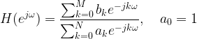
The transfer function H(e) is a pole-zero transfer function. It is best suited for modelling complex spectra having well defined resonant peaks and nulls.

Next post: Comparing AR and ARMA model – minimization of squared error

Rate this article: Note: There is a rating embedded within this post, please visit this post to rate it.

Related topics

[1]An Introduction to Estimation Theory
[2]Bias of an Estimator
[3]Minimum Variance Unbiased Estimators (MVUE)
[4]Maximum Likelihood Estimation
[5]Maximum Likelihood Decoding
[6]Probability and Random Process
[7]Likelihood Function and Maximum Likelihood Estimation (MLE)
[8]Score, Fisher Information and Estimator Sensitivity
[9]Introduction to Cramer Rao Lower Bound (CRLB)
[10]Cramer Rao Lower Bound for Scalar Parameter Estimation
[11]Applying Cramer Rao Lower Bound (CRLB) to find a Minimum Variance Unbiased Estimator (MVUE)
[12]Efficient Estimators and CRLB
[13]Cramer Rao Lower Bound for Phase Estimation
[14]Normalized CRLB - an alternate form of CRLB and its relation to estimator sensitivity
[15]Cramer Rao Lower Bound (CRLB) for Vector Parameter Estimation
[16]The Mean Square Error – Why do we use it for estimation problems
[17]How to estimate unknown parameters using Ordinary Least Squares (OLS)
[18]Essential Preliminary Matrix Algebra for Signal Processing
[19]Why Cholesky Decomposition ? A sample case:
[20]Tests for Positive Definiteness of a Matrix
[21]Solving a Triangular Matrix using Forward & Backward Substitution
[22]Cholesky Factorization - Matlab and Python
[23]LTI system models for random signals – AR, MA and ARMA models
[24]Comparing AR and ARMA model - minimization of squared error
[25]Yule Walker Estimation
[26]AutoCorrelation (Correlogram) and persistence – Time series analysis
[27]Linear Models - Least Squares Estimator (LSE)
[28]Best Linear Unbiased Estimator (BLUE)

Books by the author


Wireless Communication Systems in Matlab
Second Edition(PDF)

Note: There is a rating embedded within this post, please visit this post to rate it.
Checkout Added to cart

Digital Modulations using Python
(PDF ebook)

Note: There is a rating embedded within this post, please visit this post to rate it.
Checkout Added to cart

Digital Modulations using Matlab
(PDF ebook)

Note: There is a rating embedded within this post, please visit this post to rate it.
Checkout Added to cart
Hand-picked Best books on Communication Engineering
Best books on Signal Processing

Cramér-Rao Lower Bound (CRLB)-Vector Parameter Estimation

Key focus: Applying Cramér-Rao Lower Bound (CRLB) for vector parameter estimation. Know about covariance matrix, Fisher information matrix & CRLB matrix.

CRLB for Vector Parameter Estimation

CRLB for scalar parameter estimation was discussed in previous posts. The same concept is extended to vector parameter estimation.

Consider a set of deterministic parameters that we wish to estimate.
The estimate is denoted in vector form as, .

Assume that the estimate is unbiased .

Covariance Matrix

For the scalar parameter estimation, the variance of the estimate was considered. For vector parameter estimation, the covariance of the vector of estimates are considered.

The covariance matrix for the vector of estimates is given by

For example, if and C are the unknown parameters to be estimated, then the  covariance matrix for the parameter vector is given by


Fisher Information Matrix

For the scalar parameter estimation, Fisher Information was considered. Same concept is extended for the vector case and is called the Fisher Information Matrix . The ijth element of the Fisher Information Matrix (evaluated at the true values of the parameter vector) is given by

CRLB Matrix

Under the same regularity condition (as that of the scalar parameter estimation case),

the CRLB Matrix is given by the inverse of the Fisher Information Matrix

Note: For the scale parameter estimation, the CRLB was shown to be the reciprocal of the Fisher Information.

This implies that the covariance of the parameters (diagonal elements) are bound by the CRLB as

More generally, the condition given above is represented as

Note: The word positive-semi-definite is the matrix equivalent of saying that a value is greater than or equal to zero. Similarly, the term positive-definite is roughly equivalent of saying that something is definitely greater than zero or definitely positive.

Emphasize was place on diagonal elements in the Fisher Information Matrix. The effect of off-diagonal elements should also be considered.

For further reading

[1] Debrati et al,“A Novel Frequency Synchronization Algorithm and its Cramer Rao Bound in Practical UWB Environment for MB-OFDM Systems”, RADIOENGINEERING, VOL. 18, NO. 1, APRIL 2009.↗

Similar topics:

[1]An Introduction to Estimation Theory
[2]Bias of an Estimator
[3]Minimum Variance Unbiased Estimators (MVUE)
[4]Maximum Likelihood Estimation
[5]Maximum Likelihood Decoding
[6]Probability and Random Process
[7]Likelihood Function and Maximum Likelihood Estimation (MLE)
[8]Score, Fisher Information and Estimator Sensitivity
[9]Introduction to Cramer Rao Lower Bound (CRLB)
[10]Cramer Rao Lower Bound for Scalar Parameter Estimation
[11]Applying Cramer Rao Lower Bound (CRLB) to find a Minimum Variance Unbiased Estimator (MVUE)
[12]Efficient Estimators and CRLB
[13]Cramer Rao Lower Bound for Phase Estimation
[14]Normalized CRLB - an alternate form of CRLB and its relation to estimator sensitivity
[15]Cramer Rao Lower Bound (CRLB) for Vector Parameter Estimation
[16]The Mean Square Error – Why do we use it for estimation problems
[17]How to estimate unknown parameters using Ordinary Least Squares (OLS)
[18]Essential Preliminary Matrix Algebra for Signal Processing
[19]Why Cholesky Decomposition ? A sample case:
[20]Tests for Positive Definiteness of a Matrix
[21]Solving a Triangular Matrix using Forward & Backward Substitution
[22]Cholesky Factorization - Matlab and Python
[23]LTI system models for random signals – AR, MA and ARMA models
[24]Comparing AR and ARMA model - minimization of squared error
[25]Yule Walker Estimation
[26]AutoCorrelation (Correlogram) and persistence – Time series analysis
[27]Linear Models - Least Squares Estimator (LSE)
[28]Best Linear Unbiased Estimator (BLUE)

Books by the author:


Wireless Communication Systems in Matlab
Second Edition(PDF)

Note: There is a rating embedded within this post, please visit this post to rate it.
Checkout Added to cart

Digital Modulations using Python
(PDF ebook)

Note: There is a rating embedded within this post, please visit this post to rate it.
Checkout Added to cart

Digital Modulations using Matlab
(PDF ebook)

Note: There is a rating embedded within this post, please visit this post to rate it.
Checkout Added to cart
Hand-picked Best books on Communication Engineering
Best books on Signal Processing


Introducing The Kalman Filter

Introducing The Kalman Filter – Ramsey Faragher

PDF Text: click here

PDF Text: click here

Note: Click the playlist icon (located at the top left corner of the video frame) to watch all lectures

Video Lectures: Watch, Listen and Learn !!!

Serial #Topic Link to Video Lectures
1Advanced Matrix TheoryView Lecture
2Digital CommunicationsView Lecture
3Digital Signal Processing by Alan V. OppenheimView Lecture
4Discrete Stochastic ProcessView Lecture
5Electromagnetics and Applications View Lecture
6Error Correcting CodesView Lecture
7Fourier Transforms and Applications – Stanford UniversityView Lecture
8GPS TechnologyView Lecture
9Information Theory, Entropy and InferenceView Lecture
10Linear AlgebraView Lecture
11Low Power VLSI Circuits and SystemsView Lecture
12Signals and Systems by Alan V. OppenheimView Lecture
13Stanford Class X - Interactive ClassesView Lectures
14Wireless CommunicationsView Lecture
15MIT Open CourseWareOnline Courses
16Bayes' Theorem for Everyone - By Nat NapoletanoView Video
17Introduction to Kalman FilterView Lecture

Link will take you to external sites

Disclaimer: All the materials posted in this section are collected from various sources. GaussianWaves cannot guarantee the accuracy of the content in these video lectures. For any queries/if you would like to add a video lecture of your choice, please use the feedback form.

Cholesky decomposition: Python & Matlab

Cholesky decomposition is an efficient method for inversion of symmetric positive-definite matrices. Let’s demonstrate the method in Python and Matlab.

Cholesky factor

Any symmetric positive definite matrix can be factored as

where is lower triangular matrix. The lower triangular matrix is often called “Cholesky Factor of ”. The matrix can be interpreted as square root of the positive definite matrix .

Basic Algorithm to find Cholesky Factorization:

Note: In the following text, the variables represented in Greek letters represent scalar values, the variables represented in small Latin letters are column vectors and the variables represented in capital Latin letters are Matrices.

Given a positive definite matrix , it is partitioned as follows.

first element of and respectively
column vector at first column starting from second row of and respectively
remaining lower part of the matrix of and respectively of size

Having partitioned the matrix as shown above, the Cholesky factorization can be computed by the following iterative procedure.

Steps in computing the Cholesky factorization:

Step 1: Compute the scalar:
Step 2: Compute the column vector:
Step 3: Compute the matrix :
Step 4: Replace with , i.e,
Step 5: Repeat from step 1 till the matrix size at Step 4 becomes .

Matlab Program (implementing the above algorithm):

Function 1: [F]=cholesky(A,option)

function [F]=cholesky(A,option)
%Function to find the Cholesky factor of a Positive Definite matrix A
%Author Mathuranathan for https://www.gaussianwaves.com
%Licensed under Creative Commons: CC-NC-BY-SA 3.0
%A = positive definite matrix
%Option can be one of the following 'Lower','Upper'
%L = Cholesky factorizaton of A such that A=LL^T
%If option ='Lower', then it returns the Cholesky factored matrix L in
%lower triangular form
%If option ='Upper', then it returns the Cholesky factored matrix L in
%upper triangular form    

%Test for positive definiteness (symmetricity need to satisfy)
%Check if the matrix is symmetric
if ~isequal(A,A'),
    error('Input Matrix is not Symmetric');
end
    
if isPositiveDefinite(A),
    [m,n]=size(A);
    L=zeros(m,m);%Initialize to all zeros
    row=1;col=1;
    j=1;
    for i=1:m,
        a11=sqrt(A(1,1));
        L(row,col)=a11;
        if(m~=1), %Reached the last partition
            L21=A(j+1:m,1)/a11;
            L(row+1:end,col)=L21;
            A=(A(j+1:m,j+1:m)-L21*L21');
            [m,n]=size(A);
            row=row+1;
            col=col+1;
        end
    end
    switch nargin
        case 2
            if strcmpi(option,'upper'),F=L';
            else
                if strcmpi(option,'lower'),F=L;
                else error('Invalid option');
                end
            end
        case 1
            F=L;
        otherwise
            error('Not enough input arguments')
    end
else
        error('Given Matrix A is NOT Positive definite');
end
end

Function 2: x=isPositiveDefinite(A)

function x=isPositiveDefinite(A)
%Function to check whether a given matrix A is positive definite
%Author Mathuranathan for https://www.gaussianwaves.com
%Licensed under Creative Commons: CC-NC-BY-SA 3.0
%Returns x=1, if the input matrix is positive definite
%Returns x=0, if the input matrix is not positive definite
[m,~]=size(A);
    
%Test for positive definiteness
x=1; %Flag to check for positiveness
for i=1:m
    subA=A(1:i,1:i); %Extract upper left kxk submatrix
    if(det(subA)<=0); %Check if the determinent of the kxk submatrix is +ve
        x=0;
        break;
    end
end
%For debug
%if x, display('Given Matrix is Positive definite');
%else display('Given Matrix is NOT positive definite'); end    
end

Sample Run:

A is a randomly generated positive definite matrix. To generate a random positive definite matrix check the link in “external link” section below.

>> A=[3.3821 ,0.8784,0.3613,-2.0349; 0.8784, 2.0068, 0.5587, 0.1169; 0.3613, 0.5587, 3.6656, 0.7807; -2.0349, 0.1169, 0.7807, 2.5397];

>> cholesky(A,’Lower’) 

>> cholesky(A,’upper’) 

Python (numpy)

Let us verify the above results using Python’s Numpy package. The numpy package numpy.linalg contains the cholesky function for computing the Cholesky decomposition (returns in lower triangular matrix form). It can be summoned as follows

>>> import numpy as np

>>> A=[[3.3821 ,0.8784,0.3613,-2.0349],\
       [0.8784, 2.0068, 0.5587, 0.1169],\
       [0.3613, 0.5587, 3.6656, 0.7807],\
       [-2.0349, 0.1169, 0.7807, 2.5397]]
>>> np.linalg.cholesky(A)
>>>
array([[ 1.83904867,  0.        ,  0.        ,  0.        ],
       [ 0.47763826,  1.33366476,  0.        ,  0.        ],
       [ 0.19646027,  0.34856065,  1.87230041,  0.        ],
       [-1.106496  ,  0.48393333,  0.44298574,  0.94071184]])

Rate this article: Note: There is a rating embedded within this post, please visit this post to rate it.

Related Topics

[1]An Introduction to Estimation Theory
[2]Bias of an Estimator
[3]Minimum Variance Unbiased Estimators (MVUE)
[4]Maximum Likelihood Estimation
[5]Maximum Likelihood Decoding
[6]Probability and Random Process
[7]Likelihood Function and Maximum Likelihood Estimation (MLE)
[8]Score, Fisher Information and Estimator Sensitivity
[9]Introduction to Cramer Rao Lower Bound (CRLB)
[10]Cramer Rao Lower Bound for Scalar Parameter Estimation
[11]Applying Cramer Rao Lower Bound (CRLB) to find a Minimum Variance Unbiased Estimator (MVUE)
[12]Efficient Estimators and CRLB
[13]Cramer Rao Lower Bound for Phase Estimation
[14]Normalized CRLB - an alternate form of CRLB and its relation to estimator sensitivity
[15]Cramer Rao Lower Bound (CRLB) for Vector Parameter Estimation
[16]The Mean Square Error – Why do we use it for estimation problems
[17]How to estimate unknown parameters using Ordinary Least Squares (OLS)
[18]Essential Preliminary Matrix Algebra for Signal Processing
[19]Why Cholesky Decomposition ? A sample case:
[20]Tests for Positive Definiteness of a Matrix
[21]Solving a Triangular Matrix using Forward & Backward Substitution
[22]Cholesky Factorization - Matlab and Python
[23]LTI system models for random signals – AR, MA and ARMA models
[24]Comparing AR and ARMA model - minimization of squared error
[25]Yule Walker Estimation
[26]AutoCorrelation (Correlogram) and persistence – Time series analysis
[27]Linear Models - Least Squares Estimator (LSE)
[28]Best Linear Unbiased Estimator (BLUE)

Books by the author


Wireless Communication Systems in Matlab
Second Edition(PDF)

Note: There is a rating embedded within this post, please visit this post to rate it.
Checkout Added to cart

Digital Modulations using Python
(PDF ebook)

Note: There is a rating embedded within this post, please visit this post to rate it.
Checkout Added to cart

Digital Modulations using Matlab
(PDF ebook)

Note: There is a rating embedded within this post, please visit this post to rate it.
Checkout Added to cart
Hand-picked Best books on Communication Engineering
Best books on Signal Processing

Check Positive Definite Matrix in Matlab

Note: There is a rating embedded within this post, please visit this post to rate it.
It is often required to check if a given matrix is positive definite or not. Three methods to check the positive definiteness of a matrix were discussed in a previous article .

I will utilize the test method 2 to implement a small matlab code to check if a matrix is positive definite.The test method 2 relies on the fact that for a positive definite matrix, the determinants of all upper-left sub-matrices are positive.The following Matlab code uses an inbuilt Matlab function -‘det’ – which gives the determinant of an input matrix.

Furthermore, the successive upper \(k \times k\) sub-matrices are got by using the following notation

subA=A(1:i,1:i)

I will explain how this notation works to give the required sub-matrices.

Consider a sample matrix given below

$$ \begin{bmatrix} 1 & 2 & 3\\ 4 & 5 & 6\\ 7 & 8 & 9 \end{bmatrix}$$

The sub-matrices for the various combinations for row and column values for the above mentioned code snippet is given below

Notation Submatrix Comment
subA=A(1:1,1:1) \( \begin{bmatrix} 1 \end{bmatrix}\) Select elements from 1st row-1st column to 1st row-1st column
subA=A(1:2,1:2) \( \begin{bmatrix} 1 & 2 \\ 4 & 5 \end{bmatrix}\) Select elements from 1st row-1st column to 2nd row-2nd column
subA=A(1:3,1:3) \( \begin{bmatrix} 1 & 2 & 3\\ 4 & 5 & 6 \\ 7 & 8 & 9\end{bmatrix}\) Select elements from 1st row-1st column to 3rd row-3rd column
subA=A(1:3,1:2) \( \begin{bmatrix} 1 & 2 \\ 4 & 5 \\ 7 & 8 \end{bmatrix}\) Select elements from 1st row-1st column to 3rd row-2nd column

Matlab Code to test if a matrix is positive definite:

function x=isPositiveDefinite(A)
%Function to check whether a given matrix A is positive definite
%Author Mathuranathan for https://www.gaussianwaves.com
%Returns x=1, if the input matrix is positive definite
%Returns x=0, if the input matrix is not positive definite
%Throws error if the input matrix is not symmetric

    %Check if the matrix is symmetric
    [m,n]=size(A); 
    if m~=n,
        error('A is not Symmetric');
    end
    
    %Test for positive definiteness
    x=1; %Flag to check for positiveness
    for i=1:m
        subA=A(1:i,1:i); %Extract upper left kxk submatrix
        if(det(subA)<=0); %Check if the determinent of the kxk submatrix is +ve
            x=0;
            break;
        end
    end
    
    if x
        display('Given Matrix is Positive definite');
    else
        display('Given Matrix is NOT positive definite');
    end      
end

Sample run:

>> A=[1 2 3; 4 5 6; 7 8 9]
\(A =\begin{bmatrix}
1 & 2 & 3\\
4 & 5 & 6\\
7 & 8 & 9\end{bmatrix}\)
>> x=isPositiveDefinite(A)
Given Matrix is NOT positive definite
x = 0
------------------------------------------
>> A=[25 15 -5; 15 18 0;-5 0 11]
\(A =\begin{bmatrix}
25 & 15 & -5\\
15 & 18 & 0\\
-5 & 0 & 11 \end{bmatrix}\)
>> x=isPositiveDefinite(A)
Given Matrix is Positive definite
x = 1
------------------------------------------
>> A=[1 2 3; 4 5 6]
\(A =\begin{bmatrix}
1 & 2 & 3\\
4 & 5 & 6 \end{bmatrix}\)
>> x=isPositiveDefinite(A)
Error using isPositiveDefinite (line 11)
A is not Symmetric
------------------------------------------

Solve Triangular Matrix – Forward & Backward Substitution

Key focus: Know the expressions to solve triangular matrix using forward and backward substituting techniques and the FLOPS required for solving it.

Forward Substitution:

Consider a set of equations in a matrix form , where A is a lower triangular matrix with non-zero diagonal elements. The equation is re-written in full matrix form as

It can be solved using the following expressions

From the DSP implementation point of view, computation of requires one FLoating Point Operation per Second (FLOPS) – only one division. Computing will require 3 FLOPS – 1 multiplication, 1 division and 1 subtraction, will require 5 FLOPS – 2 multiplications, 1 division and two subtractions. Thus the computation of will require FLOPS.

Thus the overall FLOPS required for forward substitution is FLOPS

Backward substitution:

Consider a set of equations in a matrix form , where A is a upper triangular matrix with non-zero diagonal elements. The equation is re-written in full matrix form as

Solved using the following algorithm

This one also requires FLOPS.

Rate this article: Note: There is a rating embedded within this post, please visit this post to rate it.

More on Estimation Theory:

[1]An Introduction to Estimation Theory
[2]Bias of an Estimator
[3]Minimum Variance Unbiased Estimators (MVUE)
[4]Maximum Likelihood Estimation
[5]Maximum Likelihood Decoding
[6]Probability and Random Process
[7]Likelihood Function and Maximum Likelihood Estimation (MLE)
[8]Score, Fisher Information and Estimator Sensitivity
[9]Introduction to Cramer Rao Lower Bound (CRLB)
[10]Cramer Rao Lower Bound for Scalar Parameter Estimation
[11]Applying Cramer Rao Lower Bound (CRLB) to find a Minimum Variance Unbiased Estimator (MVUE)
[12]Efficient Estimators and CRLB
[13]Cramer Rao Lower Bound for Phase Estimation
[14]Normalized CRLB - an alternate form of CRLB and its relation to estimator sensitivity
[15]Cramer Rao Lower Bound (CRLB) for Vector Parameter Estimation
[16]The Mean Square Error – Why do we use it for estimation problems
[17]How to estimate unknown parameters using Ordinary Least Squares (OLS)
[18]Essential Preliminary Matrix Algebra for Signal Processing
[19]Why Cholesky Decomposition ? A sample case:
[20]Tests for Positive Definiteness of a Matrix
[21]Solving a Triangular Matrix using Forward & Backward Substitution
[22]Cholesky Factorization - Matlab and Python
[23]LTI system models for random signals – AR, MA and ARMA models
[24]Comparing AR and ARMA model - minimization of squared error
[25]Yule Walker Estimation
[26]AutoCorrelation (Correlogram) and persistence – Time series analysis
[27]Linear Models - Least Squares Estimator (LSE)
[28]Best Linear Unbiased Estimator (BLUE)

Books by the author


Wireless Communication Systems in Matlab
Second Edition(PDF)

Note: There is a rating embedded within this post, please visit this post to rate it.
Checkout Added to cart

Digital Modulations using Python
(PDF ebook)

Note: There is a rating embedded within this post, please visit this post to rate it.
Checkout Added to cart

Digital Modulations using Matlab
(PDF ebook)

Note: There is a rating embedded within this post, please visit this post to rate it.
Checkout Added to cart
Hand-picked Best books on Communication Engineering
Best books on Signal Processing

Tests for Positive Definiteness of a Matrix

In order to perform Cholesky Decomposition of a matrix, the matrix has to be a positive definite matrix. I have listed down a few simple methods to test the positive definiteness of a matrix.

Methods to test Positive Definiteness:

Remember that the term positive definiteness is valid only for symmetric matrices.

Test method 1: Existence of all Positive Pivots

For a matrix to be positive definite, all the pivots of the matrix should be positive. Hmm.. What is a pivot ?

Pivots:

Pivots are the first non-zero element in each row of a matrix that is in Row-Echelon form. Row-Echelon form of a matrix is the final resultant matrix of Gaussian Elimination technique.

In the following matrices, pivots are encircled.

A positive definite matrix will have all positive pivots. Only the second matrix shown above is a positive definite matrix. Also, it is the only symmetric matrix.

Test method 2: Determinants of all upper-left sub-matrices are positive:

Determinant of all upper-left sub-matrices must be positive.

Break the matrix in to several sub matrices, by progressively taking upper-left elements. If the determinants of all the sub-matrices are positive, then the original matrix is positive definite.

Is the following matrix Positive Definite?

Find the determinants of all possible upper sub-matrices.

Test method 3: All Positive Eigen Values

If all the Eigen values of the symmetric matrix are positive, then it is a positive definite matrix.

Is if following matrix Positive definite ?

Since, not all the Eigen Values are positive, the above matrix is NOT a positive definite matrix.

There exist several methods to determine positive definiteness of a matrix. The method listed here are simple and can be done manually for smaller matrices.

Rate this article: Note: There is a rating embedded within this post, please visit this post to rate it.

External resource:

1) Online tool to generate Eigen Values and Eigen Vectors↗

Books by the author


Wireless Communication Systems in Matlab
Second Edition(PDF)

Note: There is a rating embedded within this post, please visit this post to rate it.
Checkout Added to cart

Digital Modulations using Python
(PDF ebook)

Note: There is a rating embedded within this post, please visit this post to rate it.
Checkout Added to cart

Digital Modulations using Matlab
(PDF ebook)

Note: There is a rating embedded within this post, please visit this post to rate it.
Checkout Added to cart
Hand-picked Best books on Communication Engineering
Best books on Signal Processing

See also:

[1]An Introduction to Estimation Theory
[2]Bias of an Estimator
[3]Minimum Variance Unbiased Estimators (MVUE)
[4]Maximum Likelihood Estimation
[5]Maximum Likelihood Decoding
[6]Probability and Random Process
[7]Likelihood Function and Maximum Likelihood Estimation (MLE)
[8]Score, Fisher Information and Estimator Sensitivity
[9]Introduction to Cramer Rao Lower Bound (CRLB)
[10]Cramer Rao Lower Bound for Scalar Parameter Estimation
[11]Applying Cramer Rao Lower Bound (CRLB) to find a Minimum Variance Unbiased Estimator (MVUE)
[12]Efficient Estimators and CRLB
[13]Cramer Rao Lower Bound for Phase Estimation
[14]Normalized CRLB - an alternate form of CRLB and its relation to estimator sensitivity
[15]Cramer Rao Lower Bound (CRLB) for Vector Parameter Estimation
[16]The Mean Square Error – Why do we use it for estimation problems
[17]How to estimate unknown parameters using Ordinary Least Squares (OLS)
[18]Essential Preliminary Matrix Algebra for Signal Processing
[19]Why Cholesky Decomposition ? A sample case:
[20]Tests for Positive Definiteness of a Matrix
[21]Solving a Triangular Matrix using Forward & Backward Substitution
[22]Cholesky Factorization - Matlab and Python
[23]LTI system models for random signals – AR, MA and ARMA models
[24]Comparing AR and ARMA model - minimization of squared error
[25]Yule Walker Estimation
[26]AutoCorrelation (Correlogram) and persistence – Time series analysis
[27]Linear Models - Least Squares Estimator (LSE)
[28]Best Linear Unbiased Estimator (BLUE)

Why Cholesky Decomposition ? A sample case:

Note: There is a rating embedded within this post, please visit this post to rate it.
Matrix inversion is seen ubiquitously in signal processing applications. For example, matrix inversion is an important step in channel estimation and equalization. For instance, in GSM normal burst, 26 bits of training sequence are put in place with 114 bits of information bits. When the burst travels over the air interface (channel), it is subject to distortions due to channel effect like Inter Symbol Interference (ISI). It becomes necessary to estimate the channel impulse response (H) and equalize the effects of the channel, before attempting to decode/demodulate the information bits. The training bits are used to estimate the channel impulse response.

If the transmitted signal “x” travels over a multipath fading channel (H) with AWGN noise “w”, the received signal is modeled as

A Minimum Mean Square Error (MMSE) linear equalizer employed to cancel out the effects of ISI, attempts to minimize the error between equalizer output – “” and the transmitted signal ““. If the AWGN noise power is , then the equalizer is represented by the following equation[1].

Note that the expression involves the computation of matrix inversion – .

Matrix inversion is a tricky subject. Not all matrices are invertible. Furthermore, ordinary matrix inversion technique of finding the adjoint of a matrix and using it to invert the matrix will consume lots of memory and computation time. Physical layer algorithm (PHY) designers typically use Cholesky decomposition to invert the matrix. This helps to reduce the computational complexity of matrix inversion.

Reference:

[1] Marius Vollmer et al, ”Comparative Study of Joint Detection Technique for DS-CDMA Based Mobile Radio System”,IEEE Journal on selected areas in communications,Vol. 19, NO. 8, August

See Also:

[1]An Introduction to Estimation Theory
[2]Bias of an Estimator
[3]Minimum Variance Unbiased Estimators (MVUE)
[4]Maximum Likelihood Estimation
[5]Maximum Likelihood Decoding
[6]Probability and Random Process
[7]Likelihood Function and Maximum Likelihood Estimation (MLE)
[8]Score, Fisher Information and Estimator Sensitivity
[9]Introduction to Cramer Rao Lower Bound (CRLB)
[10]Cramer Rao Lower Bound for Scalar Parameter Estimation
[11]Applying Cramer Rao Lower Bound (CRLB) to find a Minimum Variance Unbiased Estimator (MVUE)
[12]Efficient Estimators and CRLB
[13]Cramer Rao Lower Bound for Phase Estimation
[14]Normalized CRLB - an alternate form of CRLB and its relation to estimator sensitivity
[15]Cramer Rao Lower Bound (CRLB) for Vector Parameter Estimation
[16]The Mean Square Error – Why do we use it for estimation problems
[17]How to estimate unknown parameters using Ordinary Least Squares (OLS)
[18]Essential Preliminary Matrix Algebra for Signal Processing
[19]Why Cholesky Decomposition ? A sample case:
[20]Tests for Positive Definiteness of a Matrix
[21]Solving a Triangular Matrix using Forward & Backward Substitution
[22]Cholesky Factorization - Matlab and Python
[23]LTI system models for random signals – AR, MA and ARMA models
[24]Comparing AR and ARMA model - minimization of squared error
[25]Yule Walker Estimation
[26]AutoCorrelation (Correlogram) and persistence – Time series analysis
[27]Linear Models - Least Squares Estimator (LSE)
[28]Best Linear Unbiased Estimator (BLUE)

Matrix Algebra for Signal Processing

Key focus : Essential matrix algebra: formation of matrices, determinants, rank, inverse & transpose of matrix and solving simultaneous equations.

I thought of making a post on Cholesky Decomposition, which is a very essential technique in digital signal processing applications like generating correlated random variables, solving linear equations, channel estimation etc.., But jumping straight to the topic of Cholesky Decomposition will leave many flummoxed/confused. So I decided to touch on some essentials in basic matrix algebra before taking up advanced topics.

Prerequisite:

Basic knowledge on topics like formation of matrices, determinants, rank of a matrix, inverse & transpose of matrix, solving a system of simultaneous equation using matrix algebra.

The prerequisites listed above being fulfilled, you will learn different types of matrices in this post.

1. Vector

A matrix with only one row or one column.

2. Transpose of a Matrix

Transpose of a matrix is formed by interchanging the elements from row to columns. For example, the first row of the matrix becomes first column in the transpose matrix, second row of the matrix becomes second column in the transpose matrix and so on.

3. Square Matrix:

Matrix with equal number of rows and columns.
(Note: The sample matrices shown below are of 3×3 dimension. They can be readily extended to nxn dimension)

Square Matrix is further classified into

4. Symmetric Matrix :

If a square matrix and its transpose are equal, then it is called a symmetric square matrix or simply symmetric matrix.

5. Diagonal Matrix

A special kind of symmetric matrix, with zeros in off-diagonal locations.

6. Scalar matrix

A special kind of diagonal matrix, with the equal values at the diagonal

7. Identity Matrix

It is a special type of scalar matrix, where the leading diagonals are one. It is denoted by I

8. Inverse of a Matrix or the notion of non-Singular Matrix:

Inverse matrices are defined for square matrices. For non-square matrices, inverses do not exist. The product of a square matrix and its inverse yields an identity matrix.
For a square matrix A.

Here denotes the inverse of square matrix .

It is possible to have a square matrix but not invertible. Such non-invertible square matrices are called
Singular Matrices. Matrix that are invertible are called non-singular matrices.

9. Singular Matrix:

A non-invertible square matrix. Inverse does not exist.

10. Orthogonal Matrix

An invertible square matrix, whose transpose and inverse are equal. If for an invertible square matrix A,

then, the matrix or equivalently is called an orthogonal matrix.

11. Complex Matrix :

A matrix with complex elements.

12. Complex Square Matrix

A complex matrix with with equal number of rows and columns

13. Conjugate Transpose or Hermitian Transpose:

Similar to the transpose of a matrix defined above. But the only difference is : put the complex conjugate form of the element when interchanging from rows to columns. For a complex square matrix , the conjugate transpose is denoted by

14. Hermitian Matrix:

A complex square matrix whose conjugate transpose is equal to its own. For a complex square matrix , the Hermitian Matix is denoted by . For a Hermitian matrix, the element of the complex square matrix located at i-th row and j-th column will be equal to the complex conjugate of the element located at j-th row and i-th column.

That is,

15. Triangular Matrix:

A special type of square matrix. Further classified into : lower triangular and upper triangular matrix. For a lower triangular matrix, all the elements above the main diagonal are zeros.For an upper triangular matrix, all the elements below the main diagonal are zeros.

16. Positive-Definite Matrix:

It is defined for both real matrices and complex matrices. It is matrix equivalent to positivity of real numbers. For example, the numbers +3,+5 and +6 are definitely positive. Similarly a positive definite matrix is defined to be definitely positive if it satisfies the following condition.

For real case: A n x n symmetric square real matrix – is said to be positive definite for all if and only if,

For complex case: A n x n symmetric square complex matrix – is said to be positive definite for all if and only if,

17. Positive-semi-definite Matrix:

It is defined for both real matrices and complex matrices. It is matrix equivalent to semi-positivity of real numbers. For example, the numbers +3,+5 and +6 are definitely positive. But the set is not positive definite since it includes a zero element which is neither positive nor negative. Similarly a positive semi-definite matrix is defined to be semi-definitely positive if it satisfies the following condition.

For real case: A n x n symmetric square real matrix – is said to be positive semi-definite for all if and only if,

For complex case: A n x n symmetric square complex matrix – is said to be positive semi-definite for all if and only if,

Note : The notation stands for a set of real numbers. The notation denotes a set of n real numbers in n-dimensional space.

18. Negative-Definite Matrix:

It is defined for both real matrices and complex matrices. It is matrix equivalent to negativity of real numbers. For example, the numbers -3,-5 and -6 are definitely negative. Similarly a negative definite matrix is defined to be definitely negative if it satisfies the following condition.

For real case: A n x n symmetric square real matrix – is said to be negative definite for all if and only if,

For complex case: A n x n symmetric square complex matrix – is said to be negative definite for all if and only if,

Note : The notation stands for a set of real numbers. The notation denotes a set of n real numbers in n-dimensional space.

19. Negative-semi-definite Matrix:

It is defined for both real matrices and complex matrices. It is matrix equivalent to semi-negativity of real numbers. For example, the numbers -3,-5 and -6 are definitely negative. But the set is not negative definite since it includes a zero element which is neither positive nor negative. Similarly a negative semi-definite matrix is defined to be semi-definitely negative if it satisfies the following condition.

For real case: A n x n symmetric square real matrix – is said to be negative semi-definite for all if and only if,

For complex case: A n x n symmetric square complex matrix – is said to be negative semi-definite for all if and only if,

Note : The notation stands for a set of real numbers. The notation denotes a set of n real numbers in n-dimensional space.

20. Indefinite Matrix :

A Matrix, that is neither positive definite, positive semi-definite, negative definite nor negative semi-definite is called an indefinite Matrix.

Rate this article: Note: There is a rating embedded within this post, please visit this post to rate it.

External References:

[1] Vector
[2] Transpose of a Matrix
[3] Square Matrix
[4] Symmetric Matrix
[5] Diagonal Matrix
[6] Scalar Matrix
[7] Identity Matrix
[8] Inverse Matrix
[9] Singular Matrix
[10] Orthogonal Matrix
[11] Complex Matrix
[12] Complex Square Matrix
[13] Conjugate Transpose
[14] Hermitian Matrix
[15] Triangular Matirx
[16] Positive definite, negative definite and semi-definite Matrices

Ordinary Least Squares : estimate unknown parameters

Key focus: Know how to estimate unknown parameters using Ordinary Least Squares (OLS) method.

As mentioned in the previous post, it is often required to estimate parameters that are unknown to the receiver. For example, if a fading channel is encountered in a communication system, it is desirable to estimate the channel response and cancel out the fading effects during reception.

Assumption and model selection:

For any estimation algorithm, certain assumptions have to be made. One of the main assumption is choosing an appropriate model for estimation. The chosen model should produce minimum statistical deviation and therefore should provide a “good fit”. A metric is often employed to determine the “goodness of fit”. Tests like “likelihood ratio test”, “Chi-Square test”, “Akaike Information Criterion” etc.., are used to measure the goodness of the assumed statistical model and decisions are made on the validity of the model assumption.

To keep things simple, we will consider only polynomial models.

Observed data and Least Squares estimation:

Suppose, an experiment is performed and the following data points are observed in the following table. The variable is the input to the experiment and is the output obtained. The input variable is often called “regressor”, “independent variable”, “manipulated variable”, etc. Similarly, the regression analysis jargon, the output variable or the observed variable is called “observed variable”, “explanatory variable”, “regressand” , “response variable” etc.

The aim of the experiment is to fit the experiment into a model with appropriate parameters. Once we know the model, we no longer need to perform the experiment to determine the output for any given arbitrary input. All we need to do is to use the model and generate the desired output.

Generic outline of an estimation algorithm:

We have a very small number of data points and it is four in our case. To illustrate the concept, we will choose linear model for parameter estimation. Higher order models will certainly give better performance. Remember!!! More the polynomial order, more is the number of parameters to be estimated and therefore the computational complexity will be more. It is necessary to strike a balance between the required performance and the model order.

We assume that the data points follow a linear trend. So, the linear model is chosen for the estimation problem.

Now the estimation problem simplifies to finding the parameters and . We can write the relationship between the observed variable and the input variable as

Next step is to solve for the above mentioned simultaneous equation based on least square error criterion. According to the criterion, the estimated values for and should produce minimum total squared error. Note the underlined words.

Let’s define the term – “error” for the above mentioned system of simultaneous equations. Error (which is a function of the model parameters) for one data point is the difference between the observed data and the data from the estimated model.

The sum of all squared errors is given by

Next step is to solve for and that gives minimum total squared error.

How do we find that? Employ calculus to find that. Separately take the partial derivative of with respect to and and set them to zero.

Solving the above simultaneous equations leads to the following solution

Thus, the model becomes

Solving using Matrices:

A system of simultaneous equations can be solved by Matrix manipulation. In DSP implementation of estimation algorithm, it is often convenient to work in matrix domain (especially when the number of data points becomes larger). Linear algebra is extensively used in implementing estimation algorithms on DSP processors.

The above mentioned set of data points can be represented in matrix notation as

Defining,

The set of simultaneous equations shrinks to

Given the criterion that the solution to the above equation must satisfy the minimum total squared error $latex S(\alpha)$,

The above equation simply denotes that the estimated parameter is the value of for which the error function attains the minimum.

The simultaneous equation mentioned above is a very simple case taken for illustration. For a generic case,

Usually, the above mentioned simultaneous equation may not have a unique solution. Unique solution exists if and only if all the columns of the matrix are linearly independent. Furthermore, the condition that the columns of matrix are linearly independent only means that they are orthogonal to each other. Thus the matrix is an orthogonal matrix.

For an orthogonal matrix, transpose and inverse are equivalent. That is,

Under this orthogonality condition, system of simultaneous equations become,

The solution is obtained by finding,

The aforementioned solution involves the computation of inverse of the matrix . Directly computing matrix inverses is cumbersome and computationally inefficient, especially when it comes to implementation in DSP, let alone the finite word length effects of fixed point processors. If the matrix , however large, has a very low condition number (i.e, well-conditioned) and if it is positive definite , then we can use Cholesky Decomposition to solve the equations.

This leads us to the next topic : “Cholesky Decomposition”

Rate this article: Note: There is a rating embedded within this post, please visit this post to rate it.

Related Posts

[1]An Introduction to Estimation Theory
[2]Bias of an Estimator
[3]Minimum Variance Unbiased Estimators (MVUE)
[4]Maximum Likelihood Estimation
[5]Maximum Likelihood Decoding
[6]Probability and Random Process
[7]Likelihood Function and Maximum Likelihood Estimation (MLE)
[8]Score, Fisher Information and Estimator Sensitivity
[9]Introduction to Cramer Rao Lower Bound (CRLB)
[10]Cramer Rao Lower Bound for Scalar Parameter Estimation
[11]Applying Cramer Rao Lower Bound (CRLB) to find a Minimum Variance Unbiased Estimator (MVUE)
[12]Efficient Estimators and CRLB
[13]Cramer Rao Lower Bound for Phase Estimation
[14]Normalized CRLB - an alternate form of CRLB and its relation to estimator sensitivity
[15]Cramer Rao Lower Bound (CRLB) for Vector Parameter Estimation
[16]The Mean Square Error – Why do we use it for estimation problems
[17]How to estimate unknown parameters using Ordinary Least Squares (OLS)
[18]Essential Preliminary Matrix Algebra for Signal Processing
[19]Why Cholesky Decomposition ? A sample case:
[20]Tests for Positive Definiteness of a Matrix
[21]Solving a Triangular Matrix using Forward & Backward Substitution
[22]Cholesky Factorization - Matlab and Python
[23]LTI system models for random signals – AR, MA and ARMA models
[24]Comparing AR and ARMA model - minimization of squared error
[25]Yule Walker Estimation
[26]AutoCorrelation (Correlogram) and persistence – Time series analysis
[27]Linear Models - Least Squares Estimator (LSE)
[28]Best Linear Unbiased Estimator (BLUE)

Books by the author


Wireless Communication Systems in Matlab
Second Edition(PDF)

Note: There is a rating embedded within this post, please visit this post to rate it.
Checkout Added to cart

Digital Modulations using Python
(PDF ebook)

Note: There is a rating embedded within this post, please visit this post to rate it.
Checkout Added to cart

Digital Modulations using Matlab
(PDF ebook)

Note: There is a rating embedded within this post, please visit this post to rate it.
Checkout Added to cart
Hand-picked Best books on Communication Engineering
Best books on Signal Processing