Bernoulli random variable is a discrete random variable with two outcomes – success and failure, with probabilities p and (1-p). It is a good model for binary data generators and also for modeling bit error patterns in the received binary data when a communication channel introduces random errors.
To generate a Bernoulli random variable X, in which the probability of success P(X=1)=p for some p ϵ (0,1), the discrete inverse transform method [1] can be applied on the continuous uniform random variable U(0,1) using the steps below.
● Generate uniform random number U in the interval (0,1) ● If U<p, set X=1, else set X=0
#bernoulliRV.m: Generating Bernoulli random number with success probability p
function X = bernoulliRV(L,p)
%Generate Bernoulli random number with success probability p
%L is the length of the sequence generated
U = rand(1,L); %continuous uniform random numbers in (0,1)
X = (U<p); end
Verifying law of large numbers
In probability theory, the law of large numbers is a theorem that involves repeating an experiment for a large number of times. According to this law, as the number of trials tend to become large, the average result obtained will be close to the expected value.
Let’s toss a coin with probability of heads . This experiment is repeated for a large number of times, say and the average result for each trial are calculated in a cumulative fashion.
#lawOfLargeNumbers.m: Law of large numbers illustrated using Bernoulli random variable
n=1000; %number of trials
p=0.7; %probability of success
X=bernoulliRV(n,p); %Bernoulli random variable
y_sum=sum(triu(repmat(X,[prod(size(X)) 1])')); %cumulative sum
avg = y_sum./(1:1:n); %average of results
plot(1:1:n,avg,'.'); hold on;
xlabel('Trial #'); ylabel('Probability of Heads');
plot(p*ones(1,n),'r'); legend('average','expected');
A brief intro to modeling a frequency selective fading channel using tapped delay line (TDL) filters. Rayleigh & Rician frequency-selective fading channel models explained.
Tapped delay line filters
Tapped-delay line filters (FIR filters) are best to simulate multiple echoes originating from same source. Hence they can be used to model multipath scenarios. Tapped-Delay-Line (TDL) filters with number taps can be used to simulate a multipath frequency selective fading channel. Frequency selective channels are characterized by time varying nature of the channel. For simulating a frequency selective channel, it is mandatory to have N > 1. In contrast, if N = 1, it simulates a zero-mean fading channel where all the multipath signals arrive at the receiver at the same time.
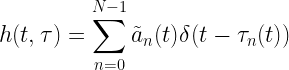
Let be the associated path attenuation corresponding to the received power and propagation delay of the th path. In continuous time, the complex path attenuation is given by
The complex channel response is given by
In the equation above, the attenuation and path delay vary with time. This simulates a time-variant complex channel.
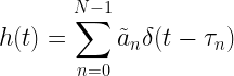
As a special case, in the absence any movements or other changes in the transmission channel, the channel can remain fairly time invariant (fixed channel with respect to instantaneous time ) even though the multipath is present. Thus the time-invariant complex channel becomes
Usually, the pair is described as a Power Delay Profile (PDP) plot. A sample power delay profile plot for a fixed, discrete, three ray model with its corresponding implementation using a tapped-delay line filter is shown in the following figure
Figure 1: 3-ray multipath time-invariant channel and its equivalent TDL implementation (path attenuations and propagation delays are fixed)
Choose underlying distribution:
The next level of modeling involves, introduction of randomness in the above mentioned model there by rendering the channel response time variant. If the path attenuations are typically drawn from a complex Gaussian random variable, then at any given time , the absolute value of the impulse response is
● Rayleigh distributed – if the mean of the distribution ● Rician distributed – if the mean of the distribution
Respectively, these two scenarios model the presence or absence of a Line of Sight (LOS) path between the transmitter and the receiver. The first propagation delay has no effect on the model behavior and hence it can be removed.
Similarly, the propagation delays can also be randomized, resulting in a more realistic but extremely complex model to implement. Furthermore, the power-delay-profile specifications with arbitrary time delays, warrant non-uniformly spaced tapped-delay-line filters, that are not suitable for practical simulation. For ease of implementation, the given PDP model with arbitrary time delays can be converted to tractable uniformly spaced statistical model by a combination of interpolation/approximation/uniform-sampling of the given power-delay-profile.
Real-life modelling:
Usually continuous domain equations for modeling multipath are specified in standards like COST-207 model in GSM specification. Such continuous time power-delay-profile models can be simulated using discrete-time Tapped Delay Line (TDL) filter with number of taps with variable tap gains. Given the order , the problem boils down to determining the discrete tap spacing and the path gains , in such a way that the simulated channel closely follows the specified multipath PDP characteristics. A survey of method to find a solution for this problem can be found in [2].
Rate this article: Note: There is a rating embedded within this post, please visit this post to rate it.
Small-scale Models for Multipath Effects
● Introduction
● Statistical characteristics of multipath channels
□ Mutipath channel models
□ Scattering function
□ Power delay profile
□ Doppler power spectrum
□ Classification of small-scale fading
● Rayleigh and Rice processes
□ Probability density function of amplitude
□ Probability density function of frequency
● Modeling frequency flat channel
● Modeling frequency selective channel
□ Method of equal distances (MED) to model specified power delay profiles
□ Simulating a frequency selective channel using TDL model
Key focus: With examples, let’s estimate and plot the probability density function of a random variable using Matlab histogram function.
Generation of random variables with required probability distribution characteristic is of paramount importance in simulating a communication system. Let’s see how we can generate a simple random variable, estimate and plot the probability density function (PDF) from the generated data and then match it with the intended theoretical PDF. Normal random variable is considered here for illustration. Other types of random variables like uniform, Bernoulli, binomial, Chi-squared, Nakagami-m are illustrated in the next section.
A survey of commonly used fundamental methods to generate a given random variable is given in [1]. For this demonstration, we will consider the normal random variable with the following parameters : – mean and – standard deviation. First generate a vector of randomly distributed random numbers of sufficient length (say 100000) with some valid values for and . There are more than one way to generate this. Some of them are given below.
● Method 1: Using the in-built random function (requires statistics toolbox)
mu=0;sigma=1;%mean=0,deviation=1
L=100000; %length of the random vector
R = random('Normal',mu,sigma,L,1);%method 1
● Method 2: Using randn function that generates normally distributed random numbers having and = 1
mu=0;sigma=1;%mean=0,deviation=1
L=100000; %length of the random vector
R = randn(L,1)*sigma + mu; %method 2
● Method 3: Box-Muller transformation [2] method using rand function that generates uniformly distributed random numbers
 mu=0;sigma=1;%mean=0,deviation=1
L=100000; %length of the random vector
U1 = rand(L,1); %uniformly distributed random numbers U(0,1)
U2 = rand(L,1); %uniformly distributed random numbers U(0,1)
Z = sqrt(-2log(U1)).cos(2piU2);%Standard Normal distribution
R = Z*sigma+mu;%Normal distribution with mean and sigma
Step 2: Plot the estimated histogram
Typically, if we have a vector of random numbers that is drawn from a distribution, we can estimate the PDF using the histogram tool. Matlab supports two in-built functions to compute and plot histograms:
● hist – introduced before R2006a ● histogram – introduced in R2014b
Which one to use ? Matlab’s help page points that the histfunction is notrecommended for several reasons and the issue of inconsistency is one among them. The histogram function is the recommended function to use.
Estimate and plot the normalized histogram using the recommended ‘histogram’ function. And for verification, overlay the theoretical PDF for the intended distribution. When using the histogram function to plot the estimated PDF from the generated random data, use ‘pdf’ option for ‘Normalization’ option. Do not use the ‘probability’ option for ‘Normalization’ option, as it will not match the theoretical PDF curve.
histogram(R,'Normalization','pdf'); %plot estimated pdf from the generated data

X = -4:0.1:4; %range of x to compute the theoretical pdf
fx_theory = pdf('Normal',X,mu,sigma); %theoretical normal probability density
hold on; plot(X,fx_theory,'r'); %plot computed theoretical PDF
title('Probability Density Function'); xlabel('values - x'); ylabel('pdf - f(x)'); axis tight;
legend('simulated','theory');
Estimated PDF (using histogram function) and the theoretical PDF
However, if you do not have Matlab version that was released before R2014b, use the ‘hist’ function and get the histogram frequency counts () and the bin-centers (). Using these data, normalize the frequency counts using the overall area under the histogram. Plot this normalized histogram and overlay the theoretical PDF for the chosen parameters.
%For those who don't have access to 'histogram' function
%get un-normalized values from hist function with same number of bins as histogram function
numBins=50; %choose appropriately
[f,x]=hist(R,numBins); %use hist function and get unnormalized values
figure; plot(x,f/trapz(x,f),'b-*');%plot normalized histogram from the generated data

X = -4:0.1:4; %range of x to compute the theoretical pdf
fx_theory =   pdf('Normal',X,mu,sigma); %theoretical normal probability density
hold on; plot(X,fx_theory,'r'); %plot computed theoretical PDF
title('Probability Density Function'); xlabel('values - x'); ylabel('pdf - f(x)'); axis tight;
legend('simulated','theory');
The given code snippets above, already include the command to plot the theoretical PDF by using the ‘pdf’ function in Matlab. It you do not have access to this function, you could use the following equation for computing the theoretical PDF
The code snippet for that purpose is given next.
X = -4:0.1:4; %range of x to compute the theoretical pdf
fx_theory = 1/sqrt(2*pi*sigma^2)*exp(-0.5*(X-mu).^2./sigma^2);
plot(X,fx_theory,'k'); %plot computed theoretical PDF
Note: The functions – ‘random’ and ‘pdf’ , requires statistics toolbox.
Rate this article: Note: There is a rating embedded within this post, please visit this post to rate it.
Root Mean Square (RMS) value is the most important parameter that signifies thesize of a signal.
Defining the term “size”:
In signal processing, a signal is viewed as a function of time. The term “size of a signal” is used to represent “strength of the signal”. It is crucial to know the “size” of a signal used in a certain application. For example, we may be interested to know the amount of electricity needed to power a LCD monitor as opposed to a CRT monitor. Both of these applications are different and have different tolerances. Thus the amount of electricity driving these devices will also be different.
A given signal’s size can be measured in many ways. Some of them are,
► Total energy ► Square root of total energy ► Integral absolute value ► Maximum or peak absolute value ► Root Mean Square (RMS) value ► Average Absolute (AA) value
Parseval’s theorem
The Parseval’s theorem expresses the energy of a signal in time-domain in terms of the average energy in its frequency components.
Suppose if the x[n] is a sequence of complex numbers of length N : xn={x0,x1,…,xN-1}, its N-point discrete Fourier transform (DFT): Xk={X0,X1,…,XN-1} is given by
The inverse discrete Fourier transform is given by
Suppose if x[n] and y[n] are two such sequences that follows the above definitions, the Parseval’s theorem is written as
where, indicates conjugate operation.
Deriving Parseval’s theorem
Energy content
Given a discrete-time sequence length N : xn={x0,x1,…,xN-1}, according to Parseval’s theorem, the energy content of the signal in the time-domain is equivalent to the average of the energy contained in its frequency components.
If the samples x[n] and X[k] are real-valued, then
Mean Square value
Mean square value is the arithmetic mean of squares of a given set of numbers. For a complex-valued signal set represented as discrete sampled values – , the mean square xMS value is given as
Applying Parseval’s theorem, the mean square value can also be computed using frequency domain components X[k]
RMS value
RMS value of a signal is calculated as the square root of average of squared value of the signal. For a complex-valued signal set represented as discrete sampled values – , the mean square xRMS value is given as
Applying Parseval’s theorem, the root mean square value can also be computed using frequency domain components X[k]
Implementing in Matlab:
Following Matlab code demonstrates the calculation of RMS value for a random sequence using time-domain and frequency domain approach. Figure 1, depicts the simulation results for RMS values for some well-known waveforms.
N=100; %length of the signal
x=randn(1,N); %a random signal to test
X=fft(x); %Frequency domain representation of the signal

RMS1 = sqrt(mean(x.*conj(x))) %RMS value from time domain samples
RMS2 = sqrt(sum(X.*conj(X))/length(x)^2) %RMS value from frequency domain representation

%Result: RMS1 = 0.9814, RMS2 = 0.9814

%Matlab has inbuilt 'rms' function, it can also be used.
Figure 1: RMS values of some well known signals
Significance of RMS value
► One of the most important parameter that is used to describe the strength of an Alternating Current (AC).
► RMS value of an AC voltage/current is equivalent to the DC voltage/current that produces the same heating effect when applied across an identical resistor. Hence, it is also a measure of energy content in a given signal.
► In statistics, for any zero-mean random stationary signal, the RMS value is same as the standard deviation of the signal. Example : Delay spread of a multipath channel is often calculated as the RMS value of the Power Delay Profile (PDP)
► When two uncorrelated (or orthogonal ) signals are added together, such as noise from two independent sources, the RMS value of their sum is equal to the square-root of sum of the square of their individual RMS values.
Rate this article: Note: There is a rating embedded within this post, please visit this post to rate it.
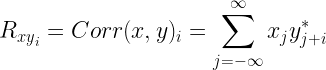
Auto-correlation, also called series correlation, is the correlation of a given sequence with itself as a function of time lag. Cross-correlation is a more generic term, which gives the correlation between two different sequences as a function of time lag.
Given two sequences and , the cross-correlation at times separated by lag i is given by ( denotes complex conjugate operation)
Auto-correlation is a special case of cross-correlation, where x=y. One can use a brute force method (using for loops implementing the above equation) to compute the auto-correlation sequence. However, other alternatives are also at your disposal.
Method 1: Auto-correlation using xcorr function
Matlab
For a N-dimensional given vector x, the Matlab command xcorr(x,x) or simply xcorr(x) gives the auto-correlation sequence. For the input sequence x=[1,2,3,4], the command xcorr(x) gives the following result.
In Python, autocorrelation of 1-D sequence can be obtained using numpy.correlate function. Set the parameter mode=’full’ which is useful for calculating the autocorrelation as a function of lag.
import numpy as np
x = np.asarray([1,2,3,4])
np.correlate(x, x,mode='full')
# output: array([ 4, 11, 20, 30, 20, 11,  4])
Method 2: Auto-correlation using Convolution
Auto-correlation sequence can be computed as the convolution between the given sequence and the reversed (flipped) version of the conjugate of the sequence.The conjugate operation is not needed if the input sequence is real.
import numpy as np
x = np.asarray([1,2,3,4])
np.convolve(x,np.conj(x)[::-1])
# output: array([ 4, 11, 20, 30, 20, 11,  4])
Method 3: Autocorrelation using Toeplitz matrix
Autocorrelation sequence can be found using Toeplitz matrices. An example for using Toeplitz matrix structure for computing convolution is given here. The same technique is extended here, where one signal is set as input sequence and the other is just the flipped version of its conjugate. The conjugate operation is not needed if the input sequence is real.
import numpy as np
from scipy.linalg import toeplitz
x = np.asarray([1,2,3,4])
toeplitz(np.pad(x, (0,len(x)-1),mode='constant'),np.pad([x[0]], (0,len(x)-1),mode='constant'))@x[::-1]
# output: array([ 4, 11, 20, 30, 20, 11, 4])
Method 4: Auto-correlation using FFT/IFFT
Auto-correlation sequence can be found using FFT/IFFT pairs. An example for using FFT/IFFT for computing convolution is given here. The same technique is extended here, where one signal is set as input sequence and the other is just the flipped version of its conjugate.The conjugate operation is not needed if the input sequence is real.
import numpy as np
from scipy.fftpack import fft,ifft

x = np.asarray([1,2,3,4])

L = 2*len(x) - 1
ifft(fft(x,L)*fft(np.conj(x)[::-1],L))
#output: array([ 4+0j, 11+0j, 20+0j, 30+0j, 20+0j, 11+0j, 4+0j])
Note that in all the above cases, due to the symmetry property of auto-correlation function, the center element represents .
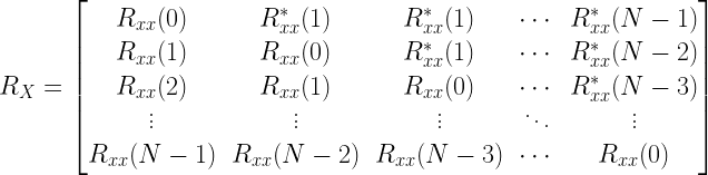
Construction the Auto-correlation Matrix
Auto-correlation matrix is a special form of matrix constructed from auto-correlation sequence. It takes the following form.
The auto-correlation matrix is easily constructed, once the auto-correlation sequence is known. The auto-correlation matrix is a Hermitian matrix as well as a Toeplitz matrix. This property is exploited in the following code for constructing the Auto-Correlation matrix.
Matlab
>> x=[1+j 2+j 3-j] %x is complex
>> acf=conv(x,fliplr(conj(x)))% %using Method 2 to compute Auto-correlation sequence
>>Rxx=acf(3:end); % R_xx(0) is the center element
>>Rx=toeplitz(Rxx,[Rxx(1) conj(Rxx(2:end))])
Python
import numpy as np
x = np.asarray([1+1j,2+1j,3-1j]) #x is complex
acf = np.convolve(x,np.conj(x)[::-1]) # using Method 2 to compute Auto-correlation sequence
Rxx=acf[2:]; # R_xx(0) is the center element
Rx = toeplitz(Rxx,np.hstack((Rxx[0], np.conj(Rxx[1:]))))
Result:
Rate this article: Note: There is a rating embedded within this post, please visit this post to rate it.
Correlation matrix defines correlation among N variables. It is a symmetric matrix with the element equal to the correlation coefficient between the and the variable. The diagonal elements (correlations of variables with themselves) are always equal to 1.
Sample problem:
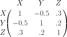
Let’s say we would like to generate three sets of random sequences X,Y,Z with the following correlation relationships.
Correlation co-efficient between X and Y is 0.5
Correlation co-efficient between X and Z is 0.3
Obviously the variable X correlates with itself 100% – i.e, correlation-coefficient is 1
Putting all these relationships in a compact matrix form, gives the correlation matrix. We take arbitrary correlation value (0.3) for the relationship between Y and Z.
Now, the task is to generate three sets of random numbers X,Y and Z that follows the relationship above. The problem can be addressed in many ways. Two most common methods finding the solution are
Generating Correlated random number using Cholesky Decomposition:
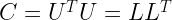
Cholesky decomposition is the matrix equivalent of taking square root operation on a given matrix. As with any scalar values, positive square root is only possible if the given number is a positive (Imaginary roots do exist otherwise). Similarly, if a matrix need to be decomposed into square-root equivalent, the matrix need to be positive definite.
The method discussed here, seeks to decompose the given correlation matrix using Cholesky decomposition.
where U and L are upper and lower triangular matrices. We will consider Upper triangular matrix here. Equivalently, lower triangular matrix can also be used, in which case the order of output needs to be reversed.
For this decomposition to work, the correlation matrix should be positive definite. The correlated random sequences (where X,Y,Z are column vectors) that follow the above relationship can be generated by multiplying the uncorrelated random numbers R with U .
Steps to follow:
Generate three sequences of uncorrelated random numbers R – each drawn from a normal distribution. For this case, the R matrix will be of size where k is the number of samples we wish to generate and we allocate the k samples in three columns, where the columns indicate the place holder for each variable X, Y and Z. Multiply this matrix with the Cholesky decomposed upper triangular version of the correlation matrix.
Python code
import numpy as np
from scipy.linalg import cholesky
from scipy.stats import pearsonr #to calculate correlation coefficient

#for plotting and visualization
import pandas as pd
import matplotlib.pyplot as plt
%matplotlib inline
plt.style.use('fivethirtyeight')
import seaborn as sns

C = np.array([[1, -0.5, 0.3],
              [-0.5, 1, 0.2],
              [0.3, 0.2, 1]]) #Construct correlation matrix
U = cholesky(C) #Cholesky decomposition
R = np.random.randn(10000,3) #Three uncorrelated sequences
Rc = R @ U #Array of correlated random sequences

#compute and display correlation coeff from generated sequences
def pearsonCorr(x, y, **kws):
    (r, _) = pearsonr(x, y) #returns Pearson’s correlation coefficient, 2-tailed p-value)
    ax = plt.gca()
    ax.annotate("r = {:.2f} ".format(r),xy=(.7, .9), xycoords=ax.transAxes)

#Visualization
df = pd.DataFrame(data=Rc, columns=['X','Y','Z'])
graph = sns.pairplot(df)
graph.map(pearsonCorr)
Figure 1: Pairplot of correlated random variables generated using Cholesky decomposition (Python)
Matlab code
x=[  1  0.5 0.3; 0.5  1  0.3; 0.3 0.3  1 ;]; %Correlation matrix
U=chol(x); %Cholesky decomposition

R=randn(10000,3); %Random data in three columns each for X,Y and Z
Rc=R*U; %Correlated matrix Rc=[X Y Z]

%Verify Correlation-Coeffs of generated vectors
coeffMatrixXX=corrcoef(Rc(:,1),Rc(:,1));
coeffMatrixXY=corrcoef(Rc(:,1),Rc(:,2));
coeffMatrixXZ=corrcoef(Rc(:,1),Rc(:,3));

%Extract the required correlation coefficients
coeffXX=coeffMatrixXX(1,2) %Correlation Coeff for XX;
coeffXY=coeffMatrixXY(1,2) %Correlation Coeff for XY;
coeffXZ=coeffMatrixXZ(1,2) %Correlation Coeff for XZ;

%Scatterplots
subplot(3,1,1)
plot(Rc(:,1),Rc(:,1),'b.')
title(['Scatterd Plot - X and X calculated \rho=' num2str(coeffXX)])
xlabel('X')
ylabel('X')

subplot(3,1,2)
plot(Rc(:,1),Rc(:,2),'r.')
title(['Scatterd Plot - X and Y calculated \rho=' num2str(coeffXY)])
xlabel('X')
ylabel('Y')

subplot(3,1,3)
plot(Rc(:,1),Rc(:,3),'m.')
title(['Scatterd Plot - X and Z calculated \rho=' num2str(coeffXZ)])
xlabel('X')
ylabel('Z')
Generating two vectors of correlated random numbers, given the correlation coefficient , is implemented in two steps. The first step is to generate two uncorrelated random sequences from an underlying distribution. Normally distributed random sequences are considered here.
A random process (or signal for your visualization) with a constant power spectral density (PSD) function is a white noise process.
Power Spectral Density
Power Spectral Density function (PSD) shows how much power is contained in each of the spectral component. For example, for a sine wave of fixed frequency, the PSD plot will contain only one spectral component present at the given frequency. PSD is an even function and so the frequency components will be mirrored across the Y-axis when plotted. Thus for a sine wave of fixed frequency, the double sided plot of PSD will have two components – one at +ve frequency and another at –ve frequency of the sine wave. (Know how to plot PSD/FFT in Python & in Matlab)
Gaussian and Uniform White Noise:
A white noise signal (process) is constituted by a set of independent and identically distributed (i.i.d) random variables. In discrete sense, the white noise signal constitutes a series of samples that are independent and generated from the same probability distribution. For example, you can generate a white noise signal using a random number generator in which all the samples follow a given Gaussian distribution. This is called White Gaussian Noise (WGN) or Gaussian White Noise. Similarly, a white noise signal generated from a Uniform distribution is called Uniform White Noise.
Gaussian Noise and Uniform Noise are frequently used in system modelling. In modelling/simulation, white noise can be generated using an appropriate random generator. White Gaussian Noise can be generated using randn function in Matlab which generates random numbers that follow a Gaussian distribution. Similarly, rand function can be used to generate Uniform White Noise in Matlab that follows a uniform distribution. When the random number generators are used, it generates a series of random numbers from the given distribution. Let’s take the example of generating a White Gaussian Noise of length 10 using randn function in Matlab – with zero mean and standard deviation=1.
This simply generates 10 random numbers from the standard normal distribution. As we know that a white process is seen as a random process composing several random variables following the same Probability Distribution Function (PDF). The 10 random numbers above are generated from the same PDF (standard normal distribution). This condition is called “identically distributed” condition. The individual samples given above are “independent” of each other. Furthermore, each sample can be viewed as a realization of one random variable. In effect, we have generated a random process that is composed of realizations of 10 random variables. Thus, the process above is constituted from “independent identically distributed” (i.i.d) random variables.
Strictly and weakly defined white noise:
Since the white noise process is constructed from i.i.d random variable/samples, all the samples follow the same underlying probability distribution function (PDF). Thus, the Joint Probability Distribution function of the process will not change with any shift in time. This is called a stationary process. Hence, this noise is a stationary process. As with a stationary process which can be classified as Strict Sense Stationary (SSS) and Wide Sense Stationary (WSS) processes, we can have white noise that is SSS and white noise that is WSS. Correspondingly they can be called strictly defined white noise signal and weakly defined white noise signal.
What’s with Covariance Function/Matrix ?
A white noise signal, denoted by \(x(t)\), is defined in weak sense is a more practical condition. Here, the samples are statistically uncorrelated and identically distributed with some variance equal to \(\sigma^2\). This condition is specified by using a covariance function as
\[COV \left(x_i, x_j \right) = \begin{cases} \sigma^2, & \quad i = j \\ 0, & \quad i \neq j \end{cases}\]
Why do we need a covariance function? Because, we are dealing with a random process that is composed of \(n\) random variables (10 variables in the modelling example above). Such a process is viewed as multivariate random vector or multivariate random variable.
For multivariate random variables, Covariance function specified how each of the \(n\) variables in the given random process behaves with respect to each other. Covariance function generalizes the notion of variance to multiple dimensions.
The above equation when represented in the matrix form gives the covariance matrix of the white noise random process. Since the random variables in this process are statistically uncorrelated, the covariance function contains values only along the diagonal.
The matrix above indicates that only the auto-correlation function exists for each random variable. The cross-correlation values are zero (samples/variables are statistically uncorrelated with respect to each other). The diagonal elements are equal to the variance and all other elements in the matrix are zero.The ensemble auto-correlation function of the weakly defined white noise is given by This indicates that the auto-correlation function of weakly defined white noise process is zero everywhere except at lag \(\tau=0\).
\[R_{xx}(\tau) = E \left[ x(t) x^*(t-\tau)\right] = \sigma^2 \delta (\tau)\]
Wiener-Khintchine Theorem states that for Wide Sense Stationary Process (WSS), the power spectral density function \(S_{xx}(f)\) of a random process can be obtained by Fourier Transform of auto-correlation function of the random process. In continuous time domain, this is represented as
\[S_{xx}(f) = F \left[R_{xx}(\tau) \right] = \int_{-\infty}^{\infty} R_{xx} (\tau) e ^{- j 2 \pi f \tau} d \tau\]
For the weakly defined white noise process, we find that the mean is a constant and its covariance does not vary with respect to time. This is a sufficient condition for a WSS process. Thus we can apply Weiner-Khintchine Theorem. Therefore, the power spectral density of the weakly defined white noise process is constant (flat) across the entire frequency spectrum (Figure 1). The value of the constant is equal to the variance or power of the noise signal.
\[S_{xx}(f) = F \left[R_{xx}(\tau) \right] = \int_{-\infty}^{\infty} \sigma^2 \delta (\tau) e ^{- j 2 \pi f \tau} d \tau = \sigma^2 \int_{-\infty}^{\infty} \delta (\tau) e ^{- j 2 \pi f \tau} = \sigma^2\]
Figure 1: Weiner-Khintchine theorem illustrated
Testing the characteristics of White Gaussian Noise in Matlab:
Generate a Gaussian white noise signal of length \(L=100,000\) using the randn function in Matlab and plot it. Let’s assume that the pdf is a Gaussian pdf with mean \(\mu=0\) and standard deviation \(\sigma=2\). Thus the variance of the Gaussian pdf is \(\sigma^2=4\). The theoretical PDF of Gaussian random variable is given by
subplot(2,1,2)
n=100; %number of Histrogram bins
[f,x]=hist(X,n);
bar(x,f/trapz(x,f)); hold on;
%Theoretical PDF of Gaussian Random Variable
g=(1/(sqrt(2*pi)*sigma))*exp(-((x-mu).^2)/(2*sigma^2));
plot(x,g);hold off; grid on;
title('Theoretical PDF and Simulated Histogram of White Gaussian Noise');
legend('Histogram','Theoretical PDF');
xlabel('Bins');
ylabel('PDF f_x(x)');
Figure 3: Plot of simulated & theoretical PDF for Gaussian RV
Compute the auto-correlation function of the white noise. The computed auto-correlation function has to be scaled properly. If the ‘xcorr’ function (inbuilt in Matlab) is used for computing the auto-correlation function, use the ‘biased’ argument in the function to scale it properly.
figure();
Rxx=1/L*conv(flipud(X),X);
lags=(-L+1):1:(L-1);

%Alternative method
%[Rxx,lags] =xcorr(X,'biased');
%The argument 'biased' is used for proper scaling by 1/L
%Normalize auto-correlation with sample length for proper scaling

plot(lags,Rxx);
title('Auto-correlation Function of white noise');
xlabel('Lags')
ylabel('Correlation')
grid on;
Figure 4: Autocorrelation function of generated noise
Simulating the PSD:
Simulating the Power Spectral Density (PSD) of the white noise is a little tricky business. There are two issues here 1) The generated samples are of finite length. This is synonymous to applying truncating an infinite series of random samples. This implies that the lags are defined over a fixed range. ( FFT and spectral leakage – an additional resource on this topic can be found here) 2) The random number generators used in simulations are pseudo-random generators. Due these two reasons, you will not get a flat spectrum of psd when you apply Fourier Transform over the generated auto-correlation values.The wavering effect of the psd can be minimized by generating sufficiently long random signal and averaging the psd over several realizations of the random signal.
Simulating Gaussian White Noise as a Multivariate Gaussian Random Vector:
To verify the power spectral density of the white noise, we will use the approach of envisaging the noise as a composite of \(N\) Gaussian random variables. We want to average the PSD over \(L\) such realizations. Since there are \(N\) Gaussian random variables (\(N\) individual samples) per realization, the covariance matrix \( C_{xx}\) will be of dimension \(N \times N\). The vector of mean for this multivariate case will be of dimension \(1 \times N\).
Cholesky decomposition of covariance matrix gives the equivalent standard deviation for the multivariate case. Cholesky decomposition can be viewed as square root operation. Matlab’s randn function is used here to generate the multi-dimensional Gaussian random process with the given mean matrix and covariance matrix.
%Verifying the constant PSD of White Gaussian Noise Process
%with arbitrary mean and standard deviation sigma

mu=0; %Mean of each realization of Noise Process
sigma=2; %Sigma of each realization of Noise Process

L = 1000; %Number of Random Signal realizations to average
N = 1024; %Sample length for each realization set as power of 2 for FFT

%Generating the Random Process - White Gaussian Noise process
MU=mu*ones(1,N); %Vector of mean for all realizations
Cxx=(sigma^2)*diag(ones(N,1)); %Covariance Matrix for the Random Process
R = chol(Cxx); %Cholesky of Covariance Matrix
%Generating a Multivariate Gaussian Distribution with given mean vector and
%Covariance Matrix Cxx
z = repmat(MU,L,1) + randn(L,N)*R;
Compute PSD of the above generated multi-dimensional process and average it to get a smooth plot.
%By default, FFT is done across each column - Normal command fft(z)
%Finding the FFT of the Multivariate Distribution across each row
%Command - fft(z,[],2)
Z = 1/sqrt(N)*fft(z,[],2); %Scaling by sqrt(N);
Pzavg = mean(Z.*conj(Z));%Computing the mean power from fft

normFreq=[-N/2:N/2-1]/N;
Pzavg=fftshift(Pzavg); %Shift zero-frequency component to center of spectrum
plot(normFreq,10*log10(Pzavg),'r');
axis([-0.5 0.5 0 10]); grid on;
ylabel('Power Spectral Density (dB/Hz)');
xlabel('Normalized Frequency');
title('Power spectral density of white noise');
Figure 5: Power spectral density of generated noise
The PSD plot of the generated noise shows almost fixed power in all the frequencies. In other words, for a white noise signal, the PSD is constant (flat) across all the frequencies (\(- \infty\) to \(+\infty\)). The y-axis in the above plot is expressed in dB/Hz unit. We can see from the plot that the \(constant \; power = 10 log_{10}(\sigma^2) = 10 log_{10}(4) = 6\; dB\).
Application
In channel modeling, we often come across additive white Gaussian noise (AWGN) channel. To know more about the channel model and its simulation, continue reading this article: Simulate AWGN channel in Matlab & Python.
Rate this article: Note: There is a rating embedded within this post, please visit this post to rate it.
Note: There is a rating embedded within this post, please visit this post to rate it.
If squares of k independent standard normal random variables are added, it gives rise to central Chi-squared distribution with ‘k’ degrees of freedom. Instead, if squares of k independent normal random variables with non-zero means are added, it gives rise to non-central Chi-squared distribution. Non-central Chi-square distribution is related to Ricean distribution, whereas the central Chi-squared distribution is related to Rayleigh distribution.
The non-central Chi-squared distribution is a generalization of Chi-square distribution. A non-central Chi squared distribution is defined by two parameters: 1) degrees of freedom () and 2) non-centrality parameter .
As we know from previous article, the degrees of freedom specify the number of independent random variables we want to square and sum-up to make the Chi-squared distribution. Non-centrality parameter is the sum of squares of means of the each independent underlying normal random variable.
The non-centrality parameter is given by
The PDF of the non-central Chi-squared distribution having degrees of freedom and non-centrality parameter is given by
Here, the random variable is central Chi-squared distributed with degrees of freedom. The factor gives the probabilities of Poisson distribution. Thus, the PDF of the non-central Chi-squared distribution can be termed as the weighted sum of Chi-squared probabilities where the weights being equal to the probabilities of Poisson distribution.
Method of Generating non-central Chi-squared random variable:
The procedure for generating the samples from a non-central Chi-squared random variable is as follows.
● For a given degree of freedom , let the normal random variables be with variances and mean respectively. ● The goal is to add squares of these independent normal random variables with variances set to one and means satisfying the condition set by equation (1). ● Set and ● Generate standard normal random variables and one normal random variable with and ● Squaring and summing-up all the random variables gives the non-central Chi-squared random variable. ● The PDF of the generated samples can be plotted using the histogram method described here.
Python numpy package has a nocentral_chisquare() generator, which can be used in a straightforward manner to obtain the non-central Chi square distributed sequences.
#---------Non-central Chi square distribution gaussianwaves.com-----
import numpy as np
import matplotlib.pyplot as plt
#%matplotlib inline
plt.style.use('ggplot')

ks=np.asarray([2,4]) #degrees of freedoms to simulate
ldas = np.asarray([1,2,3]) #non-centrality parameters to simulate
nSamp=1000000 #number of samples to generate

fig, ax = plt.subplots(ncols=1, nrows=1, constrained_layout=True)

for i,k in enumerate(ks):
    for j,lda in enumerate(ldas):
        #Generate non-central Chi-squared distributed random numbers
        X = np.random.noncentral_chisquare(df=k, nonc = lda, size = nSamp)
        ax.hist(X,bins=500,density=True,label=r'$k$={} $\lambda$={}'.format(k,lda),\
        histtype='step',alpha=0.75, linewidth=3)

ax.set_xlim(left=0,right=30);ax.legend()
ax.set_title('PDFs of non-central Chi square distribution');
plt.show()
Figure 1: Simulated PDFs of non-central Chi-Squared random variables
Rate this article: Note: There is a rating embedded within this post, please visit this post to rate it.
Note: There is a rating embedded within this post, please visit this post to rate it.
A random variable is always associated with a probability distribution. When the random variable undergoes mathematical transformation the underlying probability distribution no longer remains the same. Consider a random variable whose probability distribution function (PDF) is a standard normal distribution ( and ). Now, if the random variable is squared (a mathematical transformation), then the PDF of is no longer a standard normal distribution. The new transformed distribution is called Chi square Distribution with degree of freedom. The PDF of and are plotted in Figure 1.
Figure 1: Transformation of Normal Distribution to Chi Square Distribution
The mean of the random variable is and for the transformed variable Z2, the mean is given by . Similarly, the variance of the random variable is , whereas the variance of the transformed random variable is . In addition to the mean and variance, the shape of the distribution is also changed. The distribution of the transformed variable is no longer symmetric. In fact, the distribution is skewed to one side. Also the random variable can take only positive values whereas the random variable can take negative values too (note the x-axis in the plots above).
Since the new transformation is based on only one parameter (), the degree of freedom for this transformation is . Therefore, the transformed random variable follows – “Chi-square distribution with degree of freedom”. Suppose, if are independent random variables that follows standard normal distribution( and ), then the transformation,
is a Chi square distribution with k degrees of freedom. The following figure illustrates how the definition of the Chi square distribution as a transformation of normal distribution for degree of freedom and degrees of freedom. In the same manner, the transformation can be extended to degrees of freedom.
Figure 2: Illustration of Chi-square Distribution with 2 degrees of freedom
The above equation is derived from random variables that follow standard normal distribution. For a standard normal distribution, the mean . Therefore, the transformation is called central Chi-square distribution. If, the underlying random variables follow normal distribution with non-zero mean, then the transformation is called non-central Chi-square distribution [2] . In channel modeling, the central Chi-squared distribution is related to Rayleigh Fading scenario and the non-central Chi-square distribution is related to Rician Fading scenario.
Mathematically, the PDF of the central Chi-squared distribution with degrees of freedom is given by
The mean and variance of the central Chi-squared distributed random variable is given by
Relation to Rayleigh distribution
The connection between Chi square distribution and the Rayleigh distribution can be established as follows
If a random variable has standard Rayleigh distribution, then the transformation follows chi-square distribution with degrees of freedom.
If a random variable has the chi-square distribution with degrees of freedom, then the transformation has standard Rayleigh distribution.
Applications:
Chi-square distribution is used in hypothesis testing (to compare the observed data with expected data that follows a specific hypothesis) and in estimating variances of a parameter.
Figure 3: Simulated output – central Chi square Distribution with k degrees of freedom
Python Code
Python numpy package has achisquare() generator, which can be used in a straightforward manner to obtain the Chi square distributed sequences.
#---------Chi square distribution gaussianwaves.com-----
import numpy as np
import matplotlib.pyplot as plt
#%matplotlib inline
plt.style.use('ggplot')

ks=np.arange(start=1,stop=6,step=1) #degrees of freedoms to simulate
nSamp=1000000 #number of samples to generate

fig, ax = plt.subplots(ncols=1, nrows=1, constrained_layout=True)

for i,k in enumerate(ks):
    #Generate central Chi-square distributed random numbers
    X = np.random.chisquare(df=k, size = nSamp)
    ax.hist(X,bins=500,density=True,label=r'$k$={}'.format(k), \
    histtype='step',alpha=0.75, linewidth=3)

ax.set_xlim(left=0,right=8);ax.set_ylim(bottom=0,top=0.5);ax.legend();
ax.set_title('PDFs of Chi square distribution');
ax.set_xlabel(r'$\chi_k^2$');ax.set_ylabel(r'$f_{\chi_k^2}(x)$');
plt.show()
Rate this article: Note: There is a rating embedded within this post, please visit this post to rate it.
This website uses cookies to improve your experience while you navigate through the website. Out of these, the cookies that are categorized as necessary are stored on your browser as they are essential for the working of basic functionalities of the website. We also use third-party cookies that help us analyze and understand how you use this website. These cookies will be stored in your browser only with your consent. You also have the option to opt-out of these cookies. But opting out of some of these cookies may affect your browsing experience.
Necessary cookies are absolutely essential for the website to function properly. These cookies ensure basic functionalities and security features of the website, anonymously.
Cookie
Duration
Description
cookielawinfo-checbox-analytics
11 months
This cookie is set by GDPR Cookie Consent plugin. The cookie is used to store the user consent for the cookies in the category "Analytics".
cookielawinfo-checbox-analytics
11 months
This cookie is set by GDPR Cookie Consent plugin. The cookie is used to store the user consent for the cookies in the category "Analytics".
cookielawinfo-checbox-functional
11 months
The cookie is set by GDPR cookie consent to record the user consent for the cookies in the category "Functional".
cookielawinfo-checbox-functional
11 months
The cookie is set by GDPR cookie consent to record the user consent for the cookies in the category "Functional".
cookielawinfo-checbox-others
11 months
This cookie is set by GDPR Cookie Consent plugin. The cookie is used to store the user consent for the cookies in the category "Other.
cookielawinfo-checbox-others
11 months
This cookie is set by GDPR Cookie Consent plugin. The cookie is used to store the user consent for the cookies in the category "Other.
cookielawinfo-checkbox-necessary
11 months
This cookie is set by GDPR Cookie Consent plugin. The cookies is used to store the user consent for the cookies in the category "Necessary".
cookielawinfo-checkbox-performance
11 months
This cookie is set by GDPR Cookie Consent plugin. The cookie is used to store the user consent for the cookies in the category "Performance".
viewed_cookie_policy
11 months
The cookie is set by the GDPR Cookie Consent plugin and is used to store whether or not user has consented to the use of cookies. It does not store any personal data.
Functional cookies help to perform certain functionalities like sharing the content of the website on social media platforms, collect feedbacks, and other third-party features.
Performance cookies are used to understand and analyze the key performance indexes of the website which helps in delivering a better user experience for the visitors.
Analytical cookies are used to understand how visitors interact with the website. These cookies help provide information on metrics the number of visitors, bounce rate, traffic source, etc.


![\displaystyle{\tilde{a_n}(t) = a_n(t) exp\left[ -j 2 \pi f_c \tau_n(t) \right]}](https://s0.wp.com/latex.php?latex=%5Cdisplaystyle%7B%5Ctilde%7Ba_n%7D%28t%29+%3D+a_n%28t%29+exp%5Cleft%5B+-j+2+%5Cpi+f_c+%5Ctau_n%28t%29+%5Cright%5D%7D+&bg=ffffff&fg=000&s=2&c=20201002)


![E [h(t; \tau)] = 0](https://s0.wp.com/latex.php?latex=E+%5Bh%28t%3B+%5Ctau%29%5D+%3D+0&bg=ffffff&fg=000&s=0&c=20201002)
![E [h(t; \tau)] \neq 0](https://s0.wp.com/latex.php?latex=E+%5Bh%28t%3B+%5Ctau%29%5D+%5Cneq+0&bg=ffffff&fg=000&s=0&c=20201002)


![f_X(x) = \frac{1}{ \sqrt{ 2 \pi \sigma^2 }} exp \left[ -\frac{ \left( x-\mu \right) ^2}{2 \sigma^2} \right]](https://s0.wp.com/latex.php?latex=f_X%28x%29+%3D+%5Cfrac%7B1%7D%7B+%5Csqrt%7B+2+%5Cpi+%5Csigma%5E2+%7D%7D+exp+%5Cleft%5B+-%5Cfrac%7B+%5Cleft%28+x-%5Cmu+%5Cright%29+%5E2%7D%7B2+%5Csigma%5E2%7D+%5Cright%5D+&bg=ffffff&fg=000&s=2&c=20201002)

![X[k] = \displaystyle{\sum_{n=0}^{N-1} x[n] e^{-j\frac{2 \pi}{N} k n}}](https://s0.wp.com/latex.php?latex=X%5Bk%5D+%3D+%5Cdisplaystyle%7B%5Csum_%7Bn%3D0%7D%5E%7BN-1%7D+x%5Bn%5D+e%5E%7B-j%5Cfrac%7B2+%5Cpi%7D%7BN%7D+k+n%7D%7D+&bg=ffffff&fg=000&s=1&c=20201002)

![\tilde{x}[n] = \displaystyle{ \frac{1}{N} \sum_{k=0}^{N-1} X[k] e^{j \frac{2 \pi}{N} kn}}](https://s0.wp.com/latex.php?latex=%5Ctilde%7Bx%7D%5Bn%5D+%3D+%5Cdisplaystyle%7B+%5Cfrac%7B1%7D%7BN%7D+%5Csum_%7Bk%3D0%7D%5E%7BN-1%7D+X%5Bk%5D+e%5E%7Bj+%5Cfrac%7B2+%5Cpi%7D%7BN%7D+kn%7D%7D+&bg=ffffff&fg=000&s=1&c=20201002)

![\boxed{ \displaystyle{\sum_{n=0}^{N-1} x[n] y^{\ast}[n] = \frac{1}{N} \sum_{k=0}^{N-1} X[k] Y^{\ast}[k]}}](https://s0.wp.com/latex.php?latex=%5Cboxed%7B+%5Cdisplaystyle%7B%5Csum_%7Bn%3D0%7D%5E%7BN-1%7D+x%5Bn%5D+y%5E%7B%5Cast%7D%5Bn%5D+%3D+%5Cfrac%7B1%7D%7BN%7D+%5Csum_%7Bk%3D0%7D%5E%7BN-1%7D+X%5Bk%5D+Y%5E%7B%5Cast%7D%5Bk%5D%7D%7D+&bg=ffffff&fg=000&s=1&c=20201002)


![\begin{aligned} \sum_{n=0}^{N-1} x[n] y^{\ast}[n] &= \sum_{n=0}^{N-1} x[n] \left(\frac{1}{N} \sum_{k=0}^{N-1} Y[k] e^{j\frac{2 \pi}{N} k n} \right )^\ast \\ &= \frac{1}{N}\sum_{n=0}^{N-1} x[n] \sum_{k=0}^{N-1} Y^\ast[k] e^{-j\frac{2 \pi}{N} k n} \\ &= \frac{1}{N} \sum_{k=0}^{N-1} Y^\ast[k] \cdot \sum_{n=0}^{N-1} x[n] e^{-j\frac{2 \pi}{N} k n} \\ &= \frac{1}{N} \sum_{k=0}^{N-1} X[k] Y^\ast[k] \end{aligned}](https://s0.wp.com/latex.php?latex=%5Cbegin%7Baligned%7D+%5Csum_%7Bn%3D0%7D%5E%7BN-1%7D+x%5Bn%5D+y%5E%7B%5Cast%7D%5Bn%5D+%26%3D+%5Csum_%7Bn%3D0%7D%5E%7BN-1%7D+x%5Bn%5D+%5Cleft%28%5Cfrac%7B1%7D%7BN%7D+%5Csum_%7Bk%3D0%7D%5E%7BN-1%7D+Y%5Bk%5D+e%5E%7Bj%5Cfrac%7B2+%5Cpi%7D%7BN%7D+k+n%7D+%5Cright+%29%5E%5Cast+%5C%5C+%26%3D+%5Cfrac%7B1%7D%7BN%7D%5Csum_%7Bn%3D0%7D%5E%7BN-1%7D+x%5Bn%5D+%5Csum_%7Bk%3D0%7D%5E%7BN-1%7D+Y%5E%5Cast%5Bk%5D+e%5E%7B-j%5Cfrac%7B2+%5Cpi%7D%7BN%7D+k+n%7D+%5C%5C+%26%3D+%5Cfrac%7B1%7D%7BN%7D+%5Csum_%7Bk%3D0%7D%5E%7BN-1%7D+Y%5E%5Cast%5Bk%5D+%5Ccdot+%5Csum_%7Bn%3D0%7D%5E%7BN-1%7D+x%5Bn%5D+e%5E%7B-j%5Cfrac%7B2+%5Cpi%7D%7BN%7D+k+n%7D+%5C%5C+%26%3D+%5Cfrac%7B1%7D%7BN%7D+%5Csum_%7Bk%3D0%7D%5E%7BN-1%7D+X%5Bk%5D+Y%5E%5Cast%5Bk%5D+%5Cend%7Baligned%7D+&bg=ffffff&fg=000&s=1&c=20201002)

![\displaystyle{\sum_{n=0}^{N-1} x[n] x^\ast[n] = \frac{1}{N} \sum_{k=0}^{N-1} X[k] X^{\ast}[k]}](https://s0.wp.com/latex.php?latex=%5Cdisplaystyle%7B%5Csum_%7Bn%3D0%7D%5E%7BN-1%7D+x%5Bn%5D+x%5E%5Cast%5Bn%5D+%3D+%5Cfrac%7B1%7D%7BN%7D+%5Csum_%7Bk%3D0%7D%5E%7BN-1%7D+X%5Bk%5D+X%5E%7B%5Cast%7D%5Bk%5D%7D+&bg=ffffff&fg=000&s=1&c=20201002)

![x[n] x^\ast[n] = |x[n]|^2](https://s0.wp.com/latex.php?latex=x%5Bn%5D+x%5E%5Cast%5Bn%5D+%3D+%7Cx%5Bn%5D%7C%5E2&bg=ffffff&fg=000&s=0&c=20201002)

![\boxed{ \displaystyle{\sum_{n=0}^{N-1} \left| x[n] \right|^2 = \frac{1}{N} \sum_{k=0}^{N-1} \left| X[k] \right|^2 }}](https://s0.wp.com/latex.php?latex=%5Cboxed%7B+%5Cdisplaystyle%7B%5Csum_%7Bn%3D0%7D%5E%7BN-1%7D+%5Cleft%7C+x%5Bn%5D+%5Cright%7C%5E2+%3D+%5Cfrac%7B1%7D%7BN%7D+%5Csum_%7Bk%3D0%7D%5E%7BN-1%7D+%5Cleft%7C+X%5Bk%5D+%5Cright%7C%5E2+%7D%7D++&bg=ffffff&fg=000&s=1&c=20201002)

![[x_0,x_1,\cdots,x_{N-1}]](https://s0.wp.com/latex.php?latex=%5Bx_0%2Cx_1%2C%5Ccdots%2Cx_%7BN-1%7D%5D&bg=ffffff&fg=000&s=0&c=20201002)

![\displaystyle{ x_{MS} = \frac{ |x_0|^2 + |x_1|^2 + \cdots + |x_{N-1}|^2}{N} = \frac{1}{N} \sum_{n=0}^{N-1} |x[n]|^2 }](https://s0.wp.com/latex.php?latex=%5Cdisplaystyle%7B+x_%7BMS%7D+%3D+%5Cfrac%7B+%7Cx_0%7C%5E2+%2B+%7Cx_1%7C%5E2+%2B+%5Ccdots+%2B+%7Cx_%7BN-1%7D%7C%5E2%7D%7BN%7D+%3D+%5Cfrac%7B1%7D%7BN%7D+%5Csum_%7Bn%3D0%7D%5E%7BN-1%7D+%7Cx%5Bn%5D%7C%5E2+%7D+&bg=ffffff&fg=000&s=1&c=20201002)

![\displaystyle{ x_{MS} : \quad \frac{1}{N} \sum_{n=0}^{N-1} |x[n]|^2 = \frac{1}{N^2} \sum_{k=0}^{N-1} \left| X[k] \right|^2}](https://s0.wp.com/latex.php?latex=%5Cdisplaystyle%7B+x_%7BMS%7D+%3A+%5Cquad+%5Cfrac%7B1%7D%7BN%7D+%5Csum_%7Bn%3D0%7D%5E%7BN-1%7D+%7Cx%5Bn%5D%7C%5E2+%3D+%5Cfrac%7B1%7D%7BN%5E2%7D+%5Csum_%7Bk%3D0%7D%5E%7BN-1%7D+%5Cleft%7C+X%5Bk%5D+%5Cright%7C%5E2%7D+&bg=ffffff&fg=000&s=1&c=20201002)

![\displaystyle{ x_{RMS} = \sqrt{\frac{ |x_0|^2 + |x_1|^2 + \cdots + |x_{N-1}|^2}{N}} = \sqrt{\frac{1}{N} \sum_{n=0}^{N-1} |x[n]|^2 }}](https://s0.wp.com/latex.php?latex=%5Cdisplaystyle%7B+x_%7BRMS%7D+%3D+%5Csqrt%7B%5Cfrac%7B+%7Cx_0%7C%5E2+%2B+%7Cx_1%7C%5E2+%2B+%5Ccdots+%2B+%7Cx_%7BN-1%7D%7C%5E2%7D%7BN%7D%7D+%3D+%5Csqrt%7B%5Cfrac%7B1%7D%7BN%7D+%5Csum_%7Bn%3D0%7D%5E%7BN-1%7D+%7Cx%5Bn%5D%7C%5E2+%7D%7D+&bg=ffffff&fg=000&s=1&c=20201002)

![\displaystyle{ x_{RMS}: \quad \sqrt{\frac{1}{N} \sum_{n=0}^{N-1} |x[n]|^2} = \sqrt{\frac{1}{N^2} \sum_{k=0}^{N-1} \left| X[k] \right|^2}}](https://s0.wp.com/latex.php?latex=%5Cdisplaystyle%7B+x_%7BRMS%7D%3A+%5Cquad+%5Csqrt%7B%5Cfrac%7B1%7D%7BN%7D+%5Csum_%7Bn%3D0%7D%5E%7BN-1%7D+%7Cx%5Bn%5D%7C%5E2%7D+%3D+%5Csqrt%7B%5Cfrac%7B1%7D%7BN%5E2%7D+%5Csum_%7Bk%3D0%7D%5E%7BN-1%7D+%5Cleft%7C+X%5Bk%5D+%5Cright%7C%5E2%7D%7D+&bg=ffffff&fg=000&s=1&c=20201002)


![R_c=[X,Y, Z]](https://s0.wp.com/latex.php?latex=R_c%3D%5BX%2CY%2C+Z%5D&bg=ffffff&fg=000&s=0&c=20201002)


![\mu = E\left[\chi_k^2\right] = k](https://s0.wp.com/latex.php?latex=%5Cmu+%3D+E%5Cleft%5B%5Cchi_k%5E2%5Cright%5D+%3D+k+&bg=ffffff&fg=000&s=2&c=20201002)

![\sigma^2 = var\left[\chi_k^2\right] = 2k](https://s0.wp.com/latex.php?latex=%5Csigma%5E2+%3D+var%5Cleft%5B%5Cchi_k%5E2%5Cright%5D+%3D+2k+&bg=ffffff&fg=000&s=2&c=20201002)


