An important consideration for propagation models are the existence of objects within what is called the first Fresnel zone. Fresnel zones, referenced in Figure 1 are ellipsoids with the foci at the transmitter and the receiver, where the path length between the direct path and the alternative paths are multiples of half-wavelength (). Rays emanating from odd-numbered Fresnel zones cause destructive interference and the rays from the even-numbered Fresnel zones cause constructive interference.
As general rule of thumb for point-to-point communication, if of the first Fresnel zone is clear of obstructions, the diffraction loss would be negligible. Any further Fresnel zone clearance does not significantly alter the diffraction loss.
As an example, we would like to measure the radius of the first Fresnel zone at the midpoint between the transmitter and receiver that are separated by a distance of and operating at the frequency . The script results in the following output. The radius of the first Fresnel zone will be . It will also inform us that if at-least of the first Fresnel zone is clear of any obstruction, then any calculated diffraction loss can be safely ignored.
Program 2: FresnelzoneTest.m: Computing the diffraction loss using single knife-edge model
d=25e3; %total distance between the tx and the Rx
f=12e9; %frequency of transmission
n=1;% Freznel zone number - affects r_n only
d1=25e3/2; d2=25e3/2; %measurement at mid point
%r_n = radius of the given zone number
%r_clear = clearance required at first zone
[r_n,r_clear] = Fresnelzone(d1,d2,f,1)
Rate this article: Note: There is a rating embedded within this post, please visit this post to rate it.
Propagation environments may have obstacles that hinder the radio transmission path between the transmitter and the receiver. Idealized models for estimating the signal loss associated with diffraction by such obstacles are available. The shape of the obstacles considered in these model are too idealized for real-life applications, nevertheless, these models can serve as a good reference.
The model depicted in Figure 1 considers two idealized cases where a sharp obstacle is placed between the transmitter and the receiver. Using all the geometric parameters as indicated in the figure, the diffraction loss can be estimated with the help of a single, dimension-less quantity called Fresnel-Krichhoff diffraction parameter – . Based on the availability of information, any of the following equation can be used to calculate this parameter [1].
Figure 1: Diffracting single knife-edge obstacle having (a) positive height and (b) negative height
After computing the Fresnel-Krichhoff diffraction parameter from the geometry, the signal level due to the single knife-edge diffraction is obtained by integrating the contributions from the unhindered portions of the wavefront. The diffraction gain (or loss) is obtained as
where, and are respectively the real and imaginary part of the the complex Fresnel integral given by
The diffraction gain/loss in the equation (2) can be obtained using numerical methods which are quite involved in computation. However, for the case where , the following approximation can be used [1].
The following function implements the above approximation and can be used to compute the diffraction loss for the given Fresnel-Kirchhoff parameter.
Finally, the single knife-edge diffraction model can be coded into a function as follows. It also incorporates equation 3 (given in this post) that help us find the Fresnel zone obstructed by the given obstacle. The subject of Fresnel zones are explained in the next section.
As an example, using the sample script below, we can determine the diffraction loss incurred for , and at frequency . The computed diffraction loss will be .
Program : Computing the diffraction loss using single knife-edge model
Friis propagation model considers the line-of-sight (LOS) path between the transmitter and the receiver. The expression for the received power becomes complicated if the effect of reflections from the earth surface has to be incorporated in the modeling. In addition to the line-of-sight path, a single reflected path is added in the two ray ground reflection model, as illustrated in Figure 1. This model takes into account the phenomenon of reflection from the ground and the antenna heights above the ground. The ground surface is characterized by reflection coefficient – which depends on the material properties of the surface and the type of wave polarization. The transmitter and receiver antennas are of heights and respectively and are separated by the distance of meters.
The received signal consists of two components: LOS ray that travels the free space from the transmitter and a reflected ray from the ground surface. The distances traveled by the LOS ray and the reflected ray are given by
Depending on the phase difference () between the LOS ray and reflected ray, the received signal may suffer constructive or destructive interference. Hence, this model is also called as two ray interference model.
where, is the wavelength of the radiating wave that can be calculated from the transmission frequency. Under large-scale assumption, the power of the received signal can be expressed as
where is the product of antenna field patterns along the LOS direction and is the product of antenna field patterns along the reflected path.
The following piece of code implements equation 3 and plots the received power () against the separation distance (). The resulting plot for , , , , is shown in the Figure 2. In this plot, the transmitter power is normalized such that the plot starts at . The plot also contains approximations of the received power over three regions.
Figure 2: Distance vs received power for two ray ground reflection model and approximations**
** the approximations are shifted down in the plot for clarity, otherwise they will ride on top of the two ray model
The distance that is denoted as in the plot, is called the critical distance. It is calculated . For the region beyond the critical distance, the received power falls-off at rate. For the region where , the received power falls-off at rate and it can be approximated by free space loss equation. Table 1 captures the approximate expressions that can be applied for the three distinct regions of propagation as identified in the plot above.
Outdoor propagation models involve estimation of propagation loss over irregular terrains such as mountainous regions, simple curved earth profile, etc., with obstacles like trees and buildings. All such models predict the received signal strength at a particular distance or on a small sector. These models vary in approach, accuracy and complexity. Hata Okumura model is one such model.
In 1986, Yoshihisa Okumura traveled around Tokyo city and made measurements for the signal attenuation from base station to mobile station. He came up with a set of curves which gave the median attenuation relative to free space path loss. Okumura came up with three set of data for three scenarios: open area, urban area and sub-urban area. Since this was one of the very first model developed for cellular propagation environment, there exist other difficulties and concerns related to the applicability of the model. Okumura model can be adopted for computer simulations by digitizing those curves provided by Okumura and using them in the form of look-up-tables [1]. Since it is based on empirical studies, the validity of parameters is limited in range. The parameter values outside the range can be obtained by extrapolating the curves. There are also concerns related to the calculation of effective antenna height. Thus every RF modeling tool incorporates its own interpretations and adjustments when it comes to implementing Okumura model.
Hata, in 1980, came up with closed form expressions based on curve fitting of Okumura models. It is the most referred macroscopic propagation model. He extended the Okumura models to include effects due to diffraction, reflection and scattering of transmitted signals by the surrounding structures in a city environment.
Figure 1: Simulated distance vs. path loss using Hata model, for fc = 1500 MHz , hb = 70 m and hm = 1.5 m
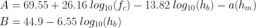
The generic closed form expression for path loss (PL) in dB scale, is given by
where, the Tx-Rx separation distance (d) is specified in kilometers (valid range 1 km to 20 Km). The factors A,B,C depend on the frequency of transmission, antenna heights and the type of environment, as given next.
● fc= frequency of transmission in MHz, valid range – 150 MHz to 1500 MHz ● hb= effective height of transmitting base station antenna in meters, valid range 30 m to 200 m ● hm=effective receiving mobile device antenna height in meters, valid range 1m to 10 m ● a(hm) = mobile antenna height correction factor that depends on the environment (refer table below) ● C = a factor used to correct the formulas for open rural and suburban areas (refer table below)
The function to simulate Hata-Okumura model is given in the book – Wireless Communication Systems using Matlab. The simulated path loss in three types of environments are plotted in Figure 1. The simulated results are obtained over a range of distances for the following parameter values fc=1500 MHz, hb=70 m and hm=1.5 m.
Rate this article: Note: There is a rating embedded within this post, please visit this post to rate it.
Radio propagation models play an important role in designing a communication system for real world applications. Propagation models are instrumental in predicting the behavior of a communication system over different environments. This chapter is aimed at providing the ideas behind the simulation of some of the subtopics in large scale propagation models, such as, free space path loss model, two ray ground reflection model, diffraction loss model and Hata-Okumura model.
Communication over a wireless network requires radio transmission and this is usually depicted as a physical layer in network stack diagrams. The physical layer defines how the data bits are transferred to and from the physical medium of the system. In case of a wireless communication system, such as wireless LAN, the radio waves are used as the link between the physical layer of a transmitter and a receiver. In this chapter, the focus is on the simulation models for modeling the physical aspects of the radio wave when they are in transit.
Radio waves are electromagnetic radiations. The branch of physics that describes the fundamental aspects of radiation is called electrodynamics. Designing a wireless equipment for interaction with an environment involves application of electrodynamics. For example, design of an antenna that produces radio waves, involves solid understanding of radiation physics.
Let’s take a simple example. The most fundamental aspect of radio waves is that it travels in all directions. A dipole antenna, the simplest and the most widely used antenna can be designed with two conducting rods. When the conducting rods are driven with the current from the transmitter, it produces radiation that travels in all directions (strength of radiation will not be uniform in all directions). By applying field equations from electrodynamics theory, it can be deduced that the strength of the radiation field decreases by in the far field, where being the distance from the antenna at which the measurement is taken. Using this result, the received power level at a given distance can be calculated and incorporated in the channel model.
Radio propagation models are broadly classified into large scale and small scale models. Large scale effects typically occur in the order of hundreds to thousands of meters in distance. Small scale effects are localized and occur temporally (in the order of a few seconds) or spatially (in the order of a few meters). This chapter is dedicated for simulation of some of the large-scale models. The small-scale simulation models are discussed in the next chapter.
The important questions in large scale modeling are – how the signal from a transmitter reaches the receiver in the first place and what is the relative power of the received signal with respect to the transmitted power level. Lots of scenarios can occur in large-scale. For example, the transmitter and the receiver could be in line-of-sight in an environment surrounded by buildings, trees and other objects. As a result, the receiver may receive – a direct attenuated signal (also called as line-of-sight (LOS) signal) from the transmitter and indirect signals (or non-line-of-sight(NLOS) signal) due to other physical effects like reflection, refraction, diffraction and scattering. The direct and indirect signals could also interfere with each other. Some of the large-scale models are briefly described here.
The Free-space propagation model is the simplest large-scale model, quite useful in satellite and microwave link modeling. It models a single unobstructed path between the transmitter and the receiver. Applying the fact that the strength of a radiation field decreases as in the far field, we arrive at theFriis free space equation that can tell us about the amount of power received relative to the power transmitted. The log distance propagation model is an extension to Friis space propagation model. It incorporates a path-loss exponent that is used to predict the relative received power in a wide range of environments.
In the absence of line-of-sight signal, other physical phenomena like refection, diffraction, etc.., must be relied upon for the modeling. Reflection involves a change in direction of the signal wavefront when it bounces off an object with different optical properties. The plane-earth loss model is another simple propagation model that considers the interaction between the line-of-sight signal and the reflected signal.
Diffraction is another phenomena in radiation physics that makes it possible for a radiated wave bend around the edges of obstacles. In the knife-edge diffraction model, the path between the transmitter and the receiver is blocked by a single sharp ridge. Approximate mathematical expressions for calculating the loss-due-to-diffraction for the case of multiple ridges were also proposed by many researchers [1][2][3][4].
Of the several available large-scale models, five are selected here for simulation:
Intersymbol interference (ISI) is a common problem in telecommunication systems, such as terrestrial television broadcasting, digital data communication systems, and cellular mobile communication systems. Dispersive effects in high-speed data transmission and multipath fading are the main reasons for ISI. To maximize the capacity, the transmission bandwidth must be extended to the entire usable bandwidth of the channel and that also leads to ISI.
To mitigate the effect of ISI, equalization techniques can be applied at the receiver side. Under the assumption of correct decisions, a zero-forcing decision feedback equalization (ZF-DFE) completely removes the ISI and leaves the white noise uncolored. It was also shown that ZF-DFE in combination with powerful coding techniques, allows transmission to approach the channel capacity [1]. DFE is adaptive and works well in the presence of spectral nulls and hence suitable for various PR channels that has spectral nulls. However, DFE suffers from error propagation and is not flexible enough to incorporate itself with powerful channel coding techniques such as trellis-coded modulation (TCM) and low-density parity codes (LDPC).
These problems can be practically mitigated by employing precodingtechniques at the transmitter side. Precoding eliminates error propagation effects at the source if the channel state information is known precisely at the transmitter. Additionally, precoding at transmitter allows coding techniques to be incorporated in the same way as for channels without ISI. In this text, a partial response (PR) signaling system is taken as an example to demonstrate the concept of precoding.
Precoding system using filters
In a PR signaling scheme, a filter is used at the transmitter to introduce a controlled amount of ISI into the signal. The introduced ISI can be compensated for, at the receiver by employing an inverse filter . In the case of PR1 signaling, the filters would be
Generally, the filter is chosen to be of FIR type and therefore its inverse at the receiver will be of IIR type. If the received signal is affected by noise, the usage of IIR filter at the receiver is prone to error propagation. Therefore, instead of compensating for the ISI at the receiver, a precoder can be implemented at the transmitter as shown in Figure 1.
Figure 1: A pre-equalization system incorporating a modulo-M precoder
Since the precoder is of IIR type, the output can become unbounded. For example, let’s filter a binary data sequence through the precoder used for PR1 signaling scheme.
The result indicates that the output becomes unbounded and some additional measure has to be taken to limit the output. Assuming M-ary signaling schemes like MPAM is used for transmission, the unbounded output of the precoder can be bounded by incorporating modulo-M operation.
Rate this article: Note: There is a rating embedded within this post, please visit this post to rate it.
Reference
[1] R. Price, Nonlinear Feedback Equalized PAM versus Capacity for Noisy Filter Channels, in Proceedings of the Int. Conference on Comm. (ICC ’72), 1972, pp. 22.12-22.17
Impulse response and frequency response of PR signaling schemes
Consider a minimum bandwidth system in which the filter is represented as a cascaded combination of a partial response filter and a minimum bandwidth filter . Since is a brick-wall filter, the frequency response of the whole system is equivalent to frequency response of the FIR filter , whose transfer function, for various partial response schemes, was listed in Table 1 in the previous post (shown below).
Table 1: Partial response signaling schemes
The hand-crafted Matlab function (given in the book) generates the overall partial response signal for the given transfer function . The function records the impulse response of the filter by sending an impulse through it. These samples are computed at each symbol sampling instants. In order to visualize the pulse shaping functions and to compute the frequency response, the impulse response of are oversampled by a factor . This converts the samples from symbol rate domain to sampling rate domain. The oversampled impulse response of filter is convolved with a sinc filter that satisfies the Nyquist first criterion. This results in the overall response of the equivalent filter (refer Figure 2 in the previous post).
The Matlab code to simulate both the impulse response and the frequency response of various PR signaling schemes, is given next (refer book for the Matlab code). The simulated results are plotted in the following Figure.
Consider the generic baseband communication system model and its equivalent representation, shown in Figure 1, where the various blocks in the system are represented as filters. To have no ISI at the symbol sampling instants, the equivalent filter should satisfy Nyquist’s first criterion.
Figure 1: A generic communication system model and its equivalent representation
If the system is ideal and noiseless, it can be characterized by samples of the desired impulse response . Let’s represent all the non-zero sample values of the desired impulse response, taken at symbol sampling spacing , as , for .
The partial response signaling model, illustrated in Figure 2, is expressed as a cascaded combination of a tapped delay line filter with tap coefficients set to and a filter with frequency response . The filter forces the desired sample values. On the other hand, the filter bandlimits the system response and at the same time it preserves the sample values from the filter . The choice of filter coefficients for the filter and the different choices for for satisfying Nyquist first criterion, result in different impulse response , but renders identical sample values in Figure 2[1].
Figure 2: A generic partial response (PR) signaling model
To have a system with minimum possible bandwidth, the filter is chosen as
The inverse Fourier transform of results in a sinc pulse. The corresponding overall impulse response of the system is given by
If the bandwidth can be relaxed, other ISI free pulse-shapers like raised cosine can be considered for the filter.
Given the nature of real world channels, it is not always desirable to satisfy Nyquist’s first criterion. For example, the channel in magnetic recording, exhibits spectral null at certain frequencies and therefore it defines the channel’s upper frequency limit. In such cases, it is very difficult to satisfy Nyquist first criterion. An alternative viable solution is to allow a controlled amount of ISI between the adjacent samples at the output of the equivalent filter shown in Figure 2. This deliberate injection of controlled amount of ISI is called partial response (PR) signaling or correlative coding.
Partial Response Signaling Schemes
Several classes of PR signaling schemes and their corresponding transfer functions represented as (where is the delay operator) are shown in Table 1. The unit delay is equal to a delay of 1 symbol duration () in a continuous time system.
A brief intro to modeling a frequency selective fading channel using tapped delay line (TDL) filters. Rayleigh & Rician frequency-selective fading channel models explained.
Tapped delay line filters
Tapped-delay line filters (FIR filters) are best to simulate multiple echoes originating from same source. Hence they can be used to model multipath scenarios. Tapped-Delay-Line (TDL) filters with number taps can be used to simulate a multipath frequency selective fading channel. Frequency selective channels are characterized by time varying nature of the channel. For simulating a frequency selective channel, it is mandatory to have N > 1. In contrast, if N = 1, it simulates a zero-mean fading channel where all the multipath signals arrive at the receiver at the same time.
Let be the associated path attenuation corresponding to the received power and propagation delay of the th path. In continuous time, the complex path attenuation is given by
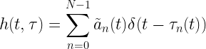
The complex channel response is given by
In the equation above, the attenuation and path delay vary with time. This simulates a time-variant complex channel.
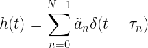
As a special case, in the absence any movements or other changes in the transmission channel, the channel can remain fairly time invariant (fixed channel with respect to instantaneous time ) even though the multipath is present. Thus the time-invariant complex channel becomes
Usually, the pair is described as a Power Delay Profile (PDP) plot. A sample power delay profile plot for a fixed, discrete, three ray model with its corresponding implementation using a tapped-delay line filter is shown in the following figure
Figure 1: 3-ray multipath time-invariant channel and its equivalent TDL implementation (path attenuations and propagation delays are fixed)
Choose underlying distribution:
The next level of modeling involves, introduction of randomness in the above mentioned model there by rendering the channel response time variant. If the path attenuations are typically drawn from a complex Gaussian random variable, then at any given time , the absolute value of the impulse response is
● Rayleigh distributed – if the mean of the distribution ● Rician distributed – if the mean of the distribution
Respectively, these two scenarios model the presence or absence of a Line of Sight (LOS) path between the transmitter and the receiver. The first propagation delay has no effect on the model behavior and hence it can be removed.
Similarly, the propagation delays can also be randomized, resulting in a more realistic but extremely complex model to implement. Furthermore, the power-delay-profile specifications with arbitrary time delays, warrant non-uniformly spaced tapped-delay-line filters, that are not suitable for practical simulation. For ease of implementation, the given PDP model with arbitrary time delays can be converted to tractable uniformly spaced statistical model by a combination of interpolation/approximation/uniform-sampling of the given power-delay-profile.
Real-life modelling:
Usually continuous domain equations for modeling multipath are specified in standards like COST-207 model in GSM specification. Such continuous time power-delay-profile models can be simulated using discrete-time Tapped Delay Line (TDL) filter with number of taps with variable tap gains. Given the order , the problem boils down to determining the discrete tap spacing and the path gains , in such a way that the simulated channel closely follows the specified multipath PDP characteristics. A survey of method to find a solution for this problem can be found in [2].
Rate this article: Note: There is a rating embedded within this post, please visit this post to rate it.
Small-scale Models for Multipath Effects
● Introduction
● Statistical characteristics of multipath channels
□ Mutipath channel models
□ Scattering function
□ Power delay profile
□ Doppler power spectrum
□ Classification of small-scale fading
● Rayleigh and Rice processes
□ Probability density function of amplitude
□ Probability density function of frequency
● Modeling frequency flat channel
● Modeling frequency selective channel
□ Method of equal distances (MED) to model specified power delay profiles
□ Simulating a frequency selective channel using TDL model
Key focus: With examples, let’s estimate and plot the probability density function of a random variable using Matlab histogram function.
Generation of random variables with required probability distribution characteristic is of paramount importance in simulating a communication system. Let’s see how we can generate a simple random variable, estimate and plot the probability density function (PDF) from the generated data and then match it with the intended theoretical PDF. Normal random variable is considered here for illustration. Other types of random variables like uniform, Bernoulli, binomial, Chi-squared, Nakagami-m are illustrated in the next section.
A survey of commonly used fundamental methods to generate a given random variable is given in [1]. For this demonstration, we will consider the normal random variable with the following parameters : – mean and – standard deviation. First generate a vector of randomly distributed random numbers of sufficient length (say 100000) with some valid values for and . There are more than one way to generate this. Some of them are given below.
● Method 1: Using the in-built random function (requires statistics toolbox)
mu=0;sigma=1;%mean=0,deviation=1
L=100000; %length of the random vector
R = random('Normal',mu,sigma,L,1);%method 1
● Method 2: Using randn function that generates normally distributed random numbers having and = 1
mu=0;sigma=1;%mean=0,deviation=1
L=100000; %length of the random vector
R = randn(L,1)*sigma + mu; %method 2
● Method 3: Box-Muller transformation [2] method using rand function that generates uniformly distributed random numbers
 mu=0;sigma=1;%mean=0,deviation=1
L=100000; %length of the random vector
U1 = rand(L,1); %uniformly distributed random numbers U(0,1)
U2 = rand(L,1); %uniformly distributed random numbers U(0,1)
Z = sqrt(-2log(U1)).cos(2piU2);%Standard Normal distribution
R = Z*sigma+mu;%Normal distribution with mean and sigma
Step 2: Plot the estimated histogram
Typically, if we have a vector of random numbers that is drawn from a distribution, we can estimate the PDF using the histogram tool. Matlab supports two in-built functions to compute and plot histograms:
● hist – introduced before R2006a ● histogram – introduced in R2014b
Which one to use ? Matlab’s help page points that the histfunction is notrecommended for several reasons and the issue of inconsistency is one among them. The histogram function is the recommended function to use.
Estimate and plot the normalized histogram using the recommended ‘histogram’ function. And for verification, overlay the theoretical PDF for the intended distribution. When using the histogram function to plot the estimated PDF from the generated random data, use ‘pdf’ option for ‘Normalization’ option. Do not use the ‘probability’ option for ‘Normalization’ option, as it will not match the theoretical PDF curve.
histogram(R,'Normalization','pdf'); %plot estimated pdf from the generated data

X = -4:0.1:4; %range of x to compute the theoretical pdf
fx_theory = pdf('Normal',X,mu,sigma); %theoretical normal probability density
hold on; plot(X,fx_theory,'r'); %plot computed theoretical PDF
title('Probability Density Function'); xlabel('values - x'); ylabel('pdf - f(x)'); axis tight;
legend('simulated','theory');
Estimated PDF (using histogram function) and the theoretical PDF
However, if you do not have Matlab version that was released before R2014b, use the ‘hist’ function and get the histogram frequency counts () and the bin-centers (). Using these data, normalize the frequency counts using the overall area under the histogram. Plot this normalized histogram and overlay the theoretical PDF for the chosen parameters.
%For those who don't have access to 'histogram' function
%get un-normalized values from hist function with same number of bins as histogram function
numBins=50; %choose appropriately
[f,x]=hist(R,numBins); %use hist function and get unnormalized values
figure; plot(x,f/trapz(x,f),'b-*');%plot normalized histogram from the generated data

X = -4:0.1:4; %range of x to compute the theoretical pdf
fx_theory =   pdf('Normal',X,mu,sigma); %theoretical normal probability density
hold on; plot(X,fx_theory,'r'); %plot computed theoretical PDF
title('Probability Density Function'); xlabel('values - x'); ylabel('pdf - f(x)'); axis tight;
legend('simulated','theory');
The given code snippets above, already include the command to plot the theoretical PDF by using the ‘pdf’ function in Matlab. It you do not have access to this function, you could use the following equation for computing the theoretical PDF
The code snippet for that purpose is given next.
X = -4:0.1:4; %range of x to compute the theoretical pdf
fx_theory = 1/sqrt(2*pi*sigma^2)*exp(-0.5*(X-mu).^2./sigma^2);
plot(X,fx_theory,'k'); %plot computed theoretical PDF
Note: The functions – ‘random’ and ‘pdf’ , requires statistics toolbox.
Rate this article: Note: There is a rating embedded within this post, please visit this post to rate it.
This website uses cookies to improve your experience while you navigate through the website. Out of these, the cookies that are categorized as necessary are stored on your browser as they are essential for the working of basic functionalities of the website. We also use third-party cookies that help us analyze and understand how you use this website. These cookies will be stored in your browser only with your consent. You also have the option to opt-out of these cookies. But opting out of some of these cookies may affect your browsing experience.
Necessary cookies are absolutely essential for the website to function properly. These cookies ensure basic functionalities and security features of the website, anonymously.
Cookie
Duration
Description
cookielawinfo-checbox-analytics
11 months
This cookie is set by GDPR Cookie Consent plugin. The cookie is used to store the user consent for the cookies in the category "Analytics".
cookielawinfo-checbox-analytics
11 months
This cookie is set by GDPR Cookie Consent plugin. The cookie is used to store the user consent for the cookies in the category "Analytics".
cookielawinfo-checbox-functional
11 months
The cookie is set by GDPR cookie consent to record the user consent for the cookies in the category "Functional".
cookielawinfo-checbox-functional
11 months
The cookie is set by GDPR cookie consent to record the user consent for the cookies in the category "Functional".
cookielawinfo-checbox-others
11 months
This cookie is set by GDPR Cookie Consent plugin. The cookie is used to store the user consent for the cookies in the category "Other.
cookielawinfo-checbox-others
11 months
This cookie is set by GDPR Cookie Consent plugin. The cookie is used to store the user consent for the cookies in the category "Other.
cookielawinfo-checkbox-necessary
11 months
This cookie is set by GDPR Cookie Consent plugin. The cookies is used to store the user consent for the cookies in the category "Necessary".
cookielawinfo-checkbox-performance
11 months
This cookie is set by GDPR Cookie Consent plugin. The cookie is used to store the user consent for the cookies in the category "Performance".
viewed_cookie_policy
11 months
The cookie is set by the GDPR Cookie Consent plugin and is used to store whether or not user has consented to the use of cookies. It does not store any personal data.
Functional cookies help to perform certain functionalities like sharing the content of the website on social media platforms, collect feedbacks, and other third-party features.
Performance cookies are used to understand and analyze the key performance indexes of the website which helps in delivering a better user experience for the visitors.
Analytical cookies are used to understand how visitors interact with the website. These cookies help provide information on metrics the number of visitors, bounce rate, traffic source, etc.


![[Q(z)]^{-1}](https://s0.wp.com/latex.php?latex=%5BQ%28z%29%5D%5E%7B-1%7D&bg=ffffff&fg=000&s=0&c=20201002)


![d_n=\left[1,0,1,0,1,0,1,0,1,0\right]](https://s0.wp.com/latex.php?latex=d_n%3D%5Cleft%5B1%2C0%2C1%2C0%2C1%2C0%2C1%2C0%2C1%2C0%5Cright%5D&bg=ffffff&fg=000&s=0&c=20201002)

![[Q(z)]^{-1}=(1+z^{-1})^{-1}](https://s0.wp.com/latex.php?latex=%5BQ%28z%29%5D%5E%7B-1%7D%3D%281%2Bz%5E%7B-1%7D%29%5E%7B-1%7D&bg=ffffff&fg=000&s=0&c=20201002)


![\displaystyle{\tilde{a_n}(t) = a_n(t) exp\left[ -j 2 \pi f_c \tau_n(t) \right]}](https://s0.wp.com/latex.php?latex=%5Cdisplaystyle%7B%5Ctilde%7Ba_n%7D%28t%29+%3D+a_n%28t%29+exp%5Cleft%5B+-j+2+%5Cpi+f_c+%5Ctau_n%28t%29+%5Cright%5D%7D+&bg=ffffff&fg=000&s=2&c=20201002)


![E [h(t; \tau)] = 0](https://s0.wp.com/latex.php?latex=E+%5Bh%28t%3B+%5Ctau%29%5D+%3D+0&bg=ffffff&fg=000&s=0&c=20201002)
![E [h(t; \tau)] \neq 0](https://s0.wp.com/latex.php?latex=E+%5Bh%28t%3B+%5Ctau%29%5D+%5Cneq+0&bg=ffffff&fg=000&s=0&c=20201002)


![f_X(x) = \frac{1}{ \sqrt{ 2 \pi \sigma^2 }} exp \left[ -\frac{ \left( x-\mu \right) ^2}{2 \sigma^2} \right]](https://s0.wp.com/latex.php?latex=f_X%28x%29+%3D+%5Cfrac%7B1%7D%7B+%5Csqrt%7B+2+%5Cpi+%5Csigma%5E2+%7D%7D+exp+%5Cleft%5B+-%5Cfrac%7B+%5Cleft%28+x-%5Cmu+%5Cright%29+%5E2%7D%7B2+%5Csigma%5E2%7D+%5Cright%5D+&bg=ffffff&fg=000&s=2&c=20201002)