GaussianWaves

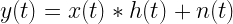
The goal of timing recovery is to estimate and correct the sampling instants and phase at the receiver, such that it allows the receiver to decode the transmitted symbols reliably.

What is Symbol timing Recovery :

When transmitting data across a communication system, three things are important: frequency of transmission, phase information and the symbol rate.

In coherent detection/demodulation, both the transmitter and receiver posses the knowledge of exact symbol sampling timing and symbol phase (and/or symbol frequency). While everything is set at the transmitter, the receiver is at the mercy of recovery algorithms to regenerate these information from the incoming signal itself. If the transmission is a passband transmission, the carrier recovery algorithm also recovers the carrier frequency. For phase sensitive systems like BPSK, QPSK etc.., the carrier recovery algorithm recovers the symbol phase so that it is synchronous with the transmitted symbol.

The first part in such a receiver architecture of a MPSK transmitting system is multiplying the incoming signal with sine and cosine components of the carrier wave.

The sine and cosine components are generated using a carrier recovery block (Phase Lock Loop (PLL) or setting a local oscillator to track the variations).

Once the in-phase and quadrature signals are separated out properly, the next task is to match each symbol with the transmitted pulse shape such that the overall SNR of the system improves.

Implementing this in digital domain, the architecture described so far would look like this (Note: the subscript of the incoming signal has changed from analog domain to digital domain – i.e. to )

In the digital architecture above, the matched filter is implemented as a simple finite impulse response (FIR) filter whose impulse response is matched to that of the transmitter pulse shape. It helps the receiver in timing recovery and also it improves the overall SNR of the system by suppressing some amount of noise. The incoming signal up to the point before the matched filter, may have fluctuations in the amplitude. The matched filter also behaves like an averaging filter that smooths out the variations in the signal.

Note that in this digital version, the incoming signal is already a sampled signal. It has already passed through an analog to digital converter that sampled the signal at some sampling rate. From the symbol perspective, the symbols have to be sampled at optimum sampling instant to extract its content properly.

This requires a re-sampler, which resamples the averaged signal at the optimum sampling instant. If the original sampling instant is before or after the optimum sampling point, the timing recovery signal will help to re-sample (re-adjust sampling times) accordingly.

Let’s take a simple BPSK transmitter for illustration. This would be equivalent to any of the single arms (in-phase and quadrature phase arms) of a QPSK transmitter or receiver.

An alternate data pattern (symbols) – [+1,-1,+1,+1,\cdots,] is transmitted across the channel. Assume that each symbol occupies T_sym=8 sample time.

clear all; clc;
n=10; %Number of data symbols
Tsym=8; %Symbol time interms of sample time or oversampling rate equivalently
%data=2*(rand(n,1)<0.5)-1;
data=[1 -1 1 -1 1 -1 1 -1 1 -1]'; %BPSK data
bpsk=reshape(repmat(data,1,Tsym)',n*Tsym,1); %BPSK signal

figure('Color',[1 1 1]);
subplot(3,1,1);
plot(bpsk);
title('Ideal BPSK symbols');
xlabel('Sample index [n]');
ylabel('Amplitude')
set(gca,'XTick',0:8:80);
axis([1 80 -2 2]); grid on;

Lets add white gaussian noise (awgn). A random noise of standard deviation 0.25 is generated and added with the generated BPSK symbols.

noise=0.25*randn(size(bpsk)); %Adding some amount of noise
received=bpsk+noise; %Received signal with noise

subplot(3,1,2);
plot(received);
title('Transmitted BPSK symbols (with noise)');
xlabel('Sample index [n]');
ylabel('Amplitude')
set(gca,'XTick',0:8:80);
axis([1 80 -2 2]); grid on;

From the first plot, we see that the transmitted pulse is a rectangular pulse that spans T_sym samples. In the illustration, T_sym=8. The best averaging filter (matched filter) for this case is a rectangular filter (though they are not preferred in practice, I am just using it for simplifying the illustration) that spans 8 samples. Such a rectangular pulse can be mathematically represented in terms of unit step function as

(Another type of averaging filter – “Moving Average Filter” is implemented here)

The resulting rectangular pulse will have a value of 0.5 at the edges of the sampling instants (index 0 and 7) and a value of ‘1’ at the remaining indices in between the edges. Such a rectangular function is indicated below.

The incoming signal is convolved with the averaging filter and the resultant output is given below

impRes=[0.5 ones(1,6) 0.5]; %Averaging Filter -> u[n]-u[n-Tsamp]
yy=conv(received,impRes,'full');
subplot(3,1,3);
plot(yy);
title('Matched Filter (Averaging Filter) output');
xlabel('Sample index [n]');
ylabel('Amplitude');

set(gca,'XTick',0:8:80);
axis([1 80 -10 10]); grid on;

We can note that the averaged output peaks at the locations where the symbol transition occurs. Thus, when the signal is sampled at those ideal locations, the BPSK symbols [+1,-1,+1, …] can be recovered perfectly.

In practice, a square root raised cosine (SRRC) filter is used both at the transmitter and the receiver (as a matched filter) to mitigate inter-symbol interference. An implementation of SRRC filter in Matlab is given here

But the problem here is: “How does the receiver know the ideal sampling instants?”. The solution is “someone has to supply those ideal sampling instants”. A symbol time recovery circuit is used for this purpose.

Coming back to the receiver architecture, lets add a symbol time recovery circuit that supplies the recovered timing instants. The signal will be re-sampled at those instants supplied by the recovery circuit.

The Algorithm behind Symbol Timing Recovery:

Different algorithms exist for symbol timing recovery and synchronization. An “Early/Late Symbol Recovery algorithm” is illustrated here.

The algorithm starts by selecting an arbitrary sample at some time (denoted by T). It captures the two adjacent samples (on either side of the sampling instant T) that are separated by δ seconds. The sample at the index T-δ is called Early Sample and the sample at the index T+δ is called Late Sample. The timing error is generated by comparing the amplitudes of the early and late samples. The next symbol sampling time instant is either advanced or delayed based on the sign of difference between the early and late sample.

1) If the Early Sample = Late Sample : The peak occurs at the on-time sampling instant T. No adjustment in the timing is needed.
2) If |Early Sample| > |Late Sample| : Late timing, the sampling time is offset so that the next symbol is sampled T-δ/2 seconds after the current sampling time.
3) If |Early Sample| < |Late Sample| : Early timing, the sampling time is offset so that the next symbol is sampled T+δ/2 seconds after the current sampling time.

These three situations are shown next.

There exist many variations to the above mentioned algorithm. The Early/Late synchronization technique given here is the simplest one taken for illustration.

Let’s complete the architecture with a signal quantization and constellation de-mapping block which gives out the estimated demodulated symbols.

Rate this article: Note: There is a rating embedded within this post, please visit this post to rate it.

For Further Reading:

[1] Technique for implementing an Early-Late Gate Synchronization structure for DPSK.↗
[2] Ying Li et al,”Hardware Implementation of Symbol Synchronization for Underwater FSK”, IEEE International Conference on Sensor Networks, Ubiquitous, and Trustworthy Computing (SUTC), p 82 – 88, 2010.↗
[3] Heinrich Meyr & Gerd Ascheid,”Digital Communication Receivers: Synchronization in Digital Communication Volume I, Phase-, Frequency-Locked Loops, and Amplitude Control (Wiley and Signal Processing)”,John Wiley & Sons; Volume 1 edition (March 1990),ISBN-13: 978-0471501930.↗
[4] Umberto Mengali,”Synchronization Techniques for Digital Receivers (Applications of Communications Theory)”,Springer; 1997 edition (October 31, 1997),ISBN-13: 978-0306457258.↗

Books by the author

Wireless Communication Systems in Matlab Second Edition(PDF) Note: There is a rating embedded within this post, please visit this post to rate it. $14.99 – Add to Cart Checkout Added to cart	Digital Modulations using Python (PDF ebook) Note: There is a rating embedded within this post, please visit this post to rate it. $14.99 – Add to Cart Checkout Added to cart	Digital Modulations using Matlab (PDF ebook) Note: There is a rating embedded within this post, please visit this post to rate it. $14.99 – Add to Cart Checkout Added to cart
Hand-picked Best books on Communication Engineering Best books on Signal Processing

References

[1] Srinivasan, S.; Haenggi, M., Path loss exponent estimation in large wireless networks, Information Theory and Applications Workshop, pp. 124 – 129, Feb 2009.↗
Topic in this chapter