Cholesky decomposition is an efficient method for inversion of symmetric positive-definite matrices. Let’s demonstrate the method in Python and Matlab.
where is lower triangular matrix. The lower triangular matrix is often called “Cholesky Factor of”. The matrix can be interpreted as square root of the positive definite matrix .
Basic Algorithm to find Cholesky Factorization:
Note: In the following text, the variables represented in Greek letters represent scalar values, the variables represented in small Latin letters are column vectors and the variables represented in capital Latin letters are Matrices.
Given a positive definite matrix , it is partitioned as follows.
first element of and respectively column vector at first column starting from second row of and respectively remaining lower part of the matrix of and respectively of size
Having partitioned the matrix as shown above, the Cholesky factorization can be computed by the following iterative procedure.
Steps in computing the Cholesky factorization:
Step 1: Compute the scalar: Step 2: Compute the column vector: Step 3: Compute the matrix : Step 4: Replace with , i.e, Step 5: Repeat from step 1 till the matrix size at Step 4 becomes .
Matlab Program (implementing the above algorithm):
Function 1: [F]=cholesky(A,option)
function [F]=cholesky(A,option)
%Function to find the Cholesky factor of a Positive Definite matrix A
%Author Mathuranathan for https://www.gaussianwaves.com
%Licensed under Creative Commons: CC-NC-BY-SA 3.0
%A = positive definite matrix
%Option can be one of the following 'Lower','Upper'
%L = Cholesky factorizaton of A such that A=LL^T
%If option ='Lower', then it returns the Cholesky factored matrix L in
%lower triangular form
%If option ='Upper', then it returns the Cholesky factored matrix L in
%upper triangular form

%Test for positive definiteness (symmetricity need to satisfy)
%Check if the matrix is symmetric
if ~isequal(A,A'),
    error('Input Matrix is not Symmetric');
end

if isPositiveDefinite(A),
    [m,n]=size(A);
    L=zeros(m,m);%Initialize to all zeros
    row=1;col=1;
    j=1;
    for i=1:m,
        a11=sqrt(A(1,1));
        L(row,col)=a11;
        if(m~=1), %Reached the last partition
            L21=A(j+1:m,1)/a11;
            L(row+1:end,col)=L21;
            A=(A(j+1:m,j+1:m)-L21*L21');
            [m,n]=size(A);
            row=row+1;
            col=col+1;
        end
    end
    switch nargin
        case 2
            if strcmpi(option,'upper'),F=L';
            else
                if strcmpi(option,'lower'),F=L;
                else error('Invalid option');
                end
            end
        case 1
            F=L;
        otherwise
            error('Not enough input arguments')
    end
else
        error('Given Matrix A is NOT Positive definite');
end
end
Function 2: x=isPositiveDefinite(A)
function x=isPositiveDefinite(A)
%Function to check whether a given matrix A is positive definite
%Author Mathuranathan for https://www.gaussianwaves.com
%Licensed under Creative Commons: CC-NC-BY-SA 3.0
%Returns x=1, if the input matrix is positive definite
%Returns x=0, if the input matrix is not positive definite
[m,~]=size(A);

%Test for positive definiteness
x=1; %Flag to check for positiveness
for i=1:m
    subA=A(1:i,1:i); %Extract upper left kxk submatrix
    if(det(subA)<=0); %Check if the determinent of the kxk submatrix is +ve
        x=0;
        break;
    end
end
%For debug
%if x, display('Given Matrix is Positive definite');
%else display('Given Matrix is NOT positive definite'); end
end
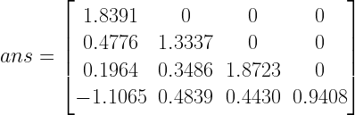
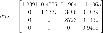
Sample Run:
A is a randomly generated positive definite matrix. To generate a random positive definite matrix check the link in “external link” section below.
Let us verify the above results using Python’s Numpy package. The numpy package numpy.linalg contains the cholesky function for computing the Cholesky decomposition (returns in lower triangular matrix form). It can be summoned as follows
Note: There is a rating embedded within this post, please visit this post to rate it.
If squares of k independent standard normal random variables are added, it gives rise to central Chi-squared distribution with ‘k’ degrees of freedom. Instead, if squares of k independent normal random variables with non-zero means are added, it gives rise to non-central Chi-squared distribution. Non-central Chi-square distribution is related to Ricean distribution, whereas the central Chi-squared distribution is related to Rayleigh distribution.
The non-central Chi-squared distribution is a generalization of Chi-square distribution. A non-central Chi squared distribution is defined by two parameters: 1) degrees of freedom () and 2) non-centrality parameter .
As we know from previous article, the degrees of freedom specify the number of independent random variables we want to square and sum-up to make the Chi-squared distribution. Non-centrality parameter is the sum of squares of means of the each independent underlying normal random variable.
The non-centrality parameter is given by
The PDF of the non-central Chi-squared distribution having degrees of freedom and non-centrality parameter is given by
Here, the random variable is central Chi-squared distributed with degrees of freedom. The factor gives the probabilities of Poisson distribution. Thus, the PDF of the non-central Chi-squared distribution can be termed as the weighted sum of Chi-squared probabilities where the weights being equal to the probabilities of Poisson distribution.
Method of Generating non-central Chi-squared random variable:
The procedure for generating the samples from a non-central Chi-squared random variable is as follows.
● For a given degree of freedom , let the normal random variables be with variances and mean respectively. ● The goal is to add squares of these independent normal random variables with variances set to one and means satisfying the condition set by equation (1). ● Set and ● Generate standard normal random variables and one normal random variable with and ● Squaring and summing-up all the random variables gives the non-central Chi-squared random variable. ● The PDF of the generated samples can be plotted using the histogram method described here.
Python numpy package has a nocentral_chisquare() generator, which can be used in a straightforward manner to obtain the non-central Chi square distributed sequences.
#---------Non-central Chi square distribution gaussianwaves.com-----
import numpy as np
import matplotlib.pyplot as plt
#%matplotlib inline
plt.style.use('ggplot')

ks=np.asarray([2,4]) #degrees of freedoms to simulate
ldas = np.asarray([1,2,3]) #non-centrality parameters to simulate
nSamp=1000000 #number of samples to generate

fig, ax = plt.subplots(ncols=1, nrows=1, constrained_layout=True)

for i,k in enumerate(ks):
    for j,lda in enumerate(ldas):
        #Generate non-central Chi-squared distributed random numbers
        X = np.random.noncentral_chisquare(df=k, nonc = lda, size = nSamp)
        ax.hist(X,bins=500,density=True,label=r'$k$={} $\lambda$={}'.format(k,lda),\
        histtype='step',alpha=0.75, linewidth=3)

ax.set_xlim(left=0,right=30);ax.legend()
ax.set_title('PDFs of non-central Chi square distribution');
plt.show()
Figure 1: Simulated PDFs of non-central Chi-Squared random variables
Rate this article: Note: There is a rating embedded within this post, please visit this post to rate it.
A generic complex baseband simulation technique, to simulate all M-ary phase shift keying (M-PSK) modulation techniques is given here. The given simulation code is very generic, and it plots both simulated and theoretical symbol error rates for all MPSK modulation techniques.
M-ary phase shift keying (M-PSK) modulation
In phase shift keying, all the information gets encoded in the phase of the carrier signal. The M-PSK modulator transmits a series of information symbols drawn from the set m∈{1,2,…,M}. Each transmitted symbol holds k bits of information (k=log2(M)). The information symbols are modulated using M-PSK mapping.
Figure 1: Signal space constellations for various MPSK modulations
The general expression for a M-PSK signal set is given by
Here, M denotes the modulation order and it defines the number of constellation points in the reference constellation. The value of M depends on the parameter k – the number of bits we wish to squeeze in a single MPSK symbol. For example if we wish to squeeze in 3 bits (k=3) in one transmit symbol, then M = 2k = 23 = 8 and this results in 8-PSK configuration. M=2 gives binary phase shift keying (BPSK) configuration. The configuration with M=4 is referred as quadrature phase shift keying (QPSK). The parameter A is the amplitude scaling factor. Using trigonometric identity, equation (1) can be separated into cosine and sine basis functions as follows
This can be expressed as a combination of in-phase and quadrature phase components on an I-Q plane as
Normalizing the amplitude as , the points on the reference constellation will be placed on the unit circle. The MPSK modulator is constructed based on this equation and the ideal constellations for M=4,8 and 16 PSK modulations are shown in Figure 1.
function [s,ref]=mpsk_modulator(M,d)
%Function to MPSK modulate the vector of data symbols - d
%[s,ref]=mpsk_modulator(M,d) modulates the symbols defined by the
%vector d using MPSK modulation, where M specifies the order of
%M-PSK modulation and the vector d contains symbols whose values
%in the range 1:M. The output s is the modulated output and ref
%represents the reference constellation that can be used in demod
   ref_i= 1/sqrt(2)*cos(((1:1:M)-1)/M*2*pi);
   ref_q= 1/sqrt(2)*sin(((1:1:M)-1)/M*2*pi);
   ref = ref_i+1i*ref_q;
   s = ref(d); %M-PSK Mapping
end
Generally the two main categories of detection techniques, commonly applied for detecting the digitally modulated data are coherent detection and non-coherent detection.
In the vector simulation model for the coherent detection, the transmitter and receiver agree on the same reference constellation for modulating and demodulating the information. The modulators generate the reference constellation for the selected modulation type. The same reference constellation should be used if coherent detection is selected as the method of demodulating the received data vector.
On the other hand, in the non-coherent detection, the receiver is oblivious to the reference constellation used at the transmitter. The receiver uses methods like envelope detection to demodulate the data.
The IQ detection technique is an example of coherent detection. In the IQ detection technique, the first step is to compute the pair-wise Euclidean distance between the given two vectors – reference array and the received symbols corrupted with noise. Each symbol in the received symbol vector (represented on a p-dimensional plane) should be compared with every symbol in the reference array. Next, the symbols, from the reference array, that provide the minimum Euclidean distance are returned.
Let x=(x1,x2,…,xp) and y=(y1,y2,…,yp) be two points in p-dimensional space. The Euclidean distance between them is given by
The pair-wise Euclidean distance between two sets of vectors, say x and y, on a p-dimensional space, can be computed using the vectorized code. The vectorized code returns the ideal signaling points from matrix y that provides the minimum Euclidean distance. Since the vectorized implementation is devoid of nested for-loops, the program executes significantly faster for larger input matrices. The given code is very generic in the sense that it can be easily reused to implement optimum coherent receivers for any N-dimensional digital modulation technique (Please refer the books Digital Modulations using Matlab and Digital Modulations using Python for complete simulation code) .
function [dCap]= mpsk_detector(M,r)
%Function to detect MPSK modulated symbols
%[dCap]= mpsk_detector(M,r) detects the received MPSK signal points
%points - 'r'. M is the modulation level of MPSK
   ref_i= 1/sqrt(2)*cos(((1:1:M)-1)/M*2*pi);
   ref_q= 1/sqrt(2)*sin(((1:1:M)-1)/M*2*pi);
   ref = ref_i+1i*ref_q; %reference constellation for MPSK
   [˜,dCap]= iqOptDetector(r,ref); %IQ detection
end
The simulation results for error rate performance of M-PSK modulations over AWGN channel and Rayleigh flat-fading channel is given in the following figures.
Figure 2: Error rate performance of MPSK modulations in AWGN channel
The moving average filter is a simple Low Pass FIR (Finite Impulse Response) filter commonly used for smoothing an array of sampled data/signal. It takes samples of input at a time and takes the average of those -samples and produces a single output point. It is a very simple LPF (Low Pass Filter) structure that comes handy for scientists and engineers to filter unwanted noisy component from the intended data.
As the filter length increases (the parameter ) the smoothness of the output increases, whereas the sharp transitions in the data are made increasingly blunt. This implies that this filter has excellent time domain response but a poor frequency response.
The MA filter performs three important functions:
1) It takes input points, computes the average of those -points and produces a single output point 2) Due to the computation/calculations involved, the filter introduces a definite amount of delay 3) The filter acts as a Low Pass Filter (with poor frequency domain response and a good time domain response).
Implementation
The difference equation for a -point discrete-time moving average filter with input represented by the vector and the averaged output vector , is
For example, a -point Moving Average FIR filter takes the current and previous four samples of input and calculates the average. This operation is represented as shown in the Figure 1 with the following difference equation for the input output relationship in discrete-time.
Figure 1: Discrete-time 5-point Moving Average FIR filter
The unit delay shown in Figure 1 is realized by either of the two options:
Representing the input samples as an array in the computer memory and processing them
Using D-Flip flop shift registers for digital hardware implementation. If each discrete value of the input is represented as a -bit signal line from ADC (analog to digital converter), then we would require 4 sets of 12-Flip flops to implement the -point moving average filter shown in Figure 1.
Z-Transform and Transfer function
In signal processing, delaying a signal by sample period (unit delay) is equivalent to multiplying the Z-transform by . By applying this idea, we can find the Z-transform of the -point moving average filter in equation (2) as
The transfer function describes the input-output relationship of the system and for the -point Moving Average filter, the transfer function is given by
where, and are the filter coefficients and the order of the filter is the maximum of and
For implementing equation (6) using the filter function, the Matlab function is called as
B = [b_0, b_1, b_2, ..., b_n] %numerator coefficients
A = [a_0, a_1, a_2, ..., a_m] %denominator coefficients
y = filter(B,A,x) %filter input x and get result in y
We can note from the difference equation and transfer function of the -point moving average filter, that following values for the numerator coefficients and denominator coefficients .
Therefore, the -point moving average filter can be coded as
B = [0.2, 0.2, 0.2, 0.2, 0.2] %numerator coefficients
A = [1] %denominator coefficients
y = filter(B,A,x) %filter input x and get result in y
The numerator coefficients for the moving average filter can be conveniently expressed in short notion as shown below
 L = 5
B = ones(1,L)/L %numerator coefficients
A = [1] %denominator coefficients
x = rand(1,10) %random samples for x
y = filter(B,A,x) %filter input x and get result in y
When using conv function to implement the moving average filter, the following code can be used
L = 5;
x = rand(1,10) %random samples for x;
y = conv(x,ones(1,L)/L)
There exists a difference between using conv function and filter function for implementing an FIR filter. The conv function gives the result of complete convolution and the length of the result is length(x)+ L -1. Whereas, the filter function gives the output that is of same length as that of the input .
In python, the filtering operation can be performed using the lfilter and convolve functions available in the scipy signal processing package. The equivalent python code is shown below.
import numpy as np
from scipy import signal
L=5 #L-point filter
b = (np.ones(L))/L #numerator co-effs of filter transfer function
a = np.ones(1)  #denominator co-effs of filter transfer function
x = np.random.randn(10) #10 random samples for x
y = signal.convolve(x,b) #filter output using convolution

y = signal.lfilter(b,a,x) #filter output using lfilter function
Pole-zero plot and frequency response
A pole-zero plot for a filter transfer function , displays the pole and zero locations in the z-plane. In the pole-zero plot, the zeros occur at locations (frequencies) where and the poles occur at locations (frequencies) where . Equivalently, zeros occurs at frequencies for which the numerator of the transfer function in equation 6 becomes zero and the poles occurs at frequencies for which the denominator of the transfer function becomes zero.
In a pole-zero plot, the locations of the poles are usually marked by cross () and the zeros are marked as circles (). The poles and zeros of a transfer function effectively define the system response and determines the stability and performance of the filtering system.
In Matlab, the pole-zero plot and the frequency response of the -point moving average can be obtained as follows.
L=11
zplane([ones(1,L)]/L,1); %pole-zero plot
w = -pi:(pi/100):pi; %to plot frequency response
freqz([ones(1,L)]/L,1,w); %plot magnitude and phase response
Figure 2: Pole-Zero plot for L=11-point Moving Average filter
Figure 3: Magnitude and phase response of L=11-point Moving Average filter
The magnitude and phase frequency responses can be coded in Python as follows
import numpy as np
from scipy import signal
import matplotlib.pyplot as plt

L=11 #L-point filter
b = (np.ones(L))/L #numerator co-effs of filter transfer function
a = np.ones(1)  #denominator co-effs of filter transfer function

w, h = signal.freqz(b,a)
plt.subplot(2, 1, 1)
plt.plot(w, 20 * np.log10(abs(h)))
plt.ylabel('Magnitude [dB]')
plt.xlabel('Frequency [rad/sample]')

plt.subplot(2, 1, 2)
angles = np.unwrap(np.angle(h))
plt.plot(w, angles)
plt.ylabel('Angle (radians)')
plt.xlabel('Frequency [rad/sample]')
plt.show()
Figure 4: Impulse response, Pole-zero plot, magnitude and phase response of L=11 moving average filter
Case study:
Following figures depict the time domain & frequency domain responses of a -point Moving Average filter. A noisy square wave signal is driven through the filter and the time domain response is obtained.
Figure 5: Processing a signal through Moving average filter of various lengths
On the first plot, we have the noisy square wave signal that is going into the moving average filter. The input is noisy and our objective is to reduce the noise as much as possible. The next figure is the output response of a 3-point Moving Average filter. It can be deduced from the figure that the 3-point Moving Average filter has not done much in filtering out the noise. We increase the filter taps to 10-points and we can see that the noise in the output has reduced a lot, which is depicted in next figure.
With L=51 tap filter, though the noise is almost zero, the transitions are blunted out drastically (observe the slope on the either side of the signal and compare them with the ideal brick wall transitions in the input signal).
From the frequency response of lower order filters (L=3, L=10), it can be asserted that the roll-off is very slow and the stop band attenuation is not good. Given this stop band attenuation, clearly, the moving average filter cannot separate one band of frequencies from another. As we increase the filter order to 51, the transitions are not preserved in time domain. Good performance in the time domain results in poor performance in the frequency domain, and vice versa. Compromise need for optimal filter design.
Rate this article: Note: There is a rating embedded within this post, please visit this post to rate it.
Quadrature Phase Shift Keying (QPSK) is a form of phase modulation technique, in which two information bits (combined as one symbol) are modulated at once, selecting one of the four possible carrier phase shift states.
Figure 1: Waveform simulation model for QPSK modulation
The QPSK signal within a symbol duration \(T_{sym}\) is defined as
\[s(t) = A \cdot cos \left[2 \pi f_c t + \theta_n \right], \quad \quad 0 \leq t \leq T_{sym},\; n=1,2,3,4 \quad \quad (1) \]
Therefore, the four possible initial signal phases are \(\pi/4, 3 \pi/4, 5 \pi/4\) and \(7 \pi/4\) radians. Equation (1) can be re-written as
\[\begin{align} s(t) &= A \cdot cos \theta_n \cdot cos \left( 2 \pi f_c t\right) – A \cdot sin \theta_n \cdot sin \left( 2 \pi f_c t\right) \\ &= s_{ni} \phi_i(t) + s_{nq} \phi_q(t) \quad\quad \quad \quad \quad\quad \quad \quad \quad\quad \quad \quad \quad\quad \quad \quad (3) \end{align} \]
The above expression indicates the use of two orthonormal basis functions: \( \left\langle \phi_i(t),\phi_q(t)\right\rangle\) together with the inphase and quadrature signaling points: \( \left\langle s_{ni}, s_{nq}\right\rangle\). Therefore, on a two dimensional co-ordinate system with the axes set to \( \phi_i(t)\) and \(\phi_q(t)\), the QPSK signal is represented by four constellation points dictated by the vectors \(\left\langle s_{ni}, s_{nq}\right\rangle\) with \( n=1,2,3,4\).
The QPSK transmitter, shown in Figure 1, is implemented as a matlab function qpsk_mod. In this implementation, a splitter separates the odd and even bits from the generated information bits. Each stream of odd bits (quadrature arm) and even bits (in-phase arm) are converted to NRZ format in a parallel manner.
function [s,t,I,Q] = qpsk_mod(a,fc,OF)
%Modulate an incoming binary stream using conventional QPSK
%a - input binary data stream (0's and 1's) to modulate
%fc - carrier frequency in Hertz
%OF - oversampling factor (multiples of fc) - at least 4 is better
%s - QPSK modulated signal with carrier
%t - time base for the carrier modulated signal
%I - baseband I channel waveform (no carrier)
%Q - baseband Q channel waveform (no carrier)
L = 2*OF;%samples in each symbol (QPSK has 2 bits in each symbol)
ak = 2*a-1; %NRZ encoding 0-> -1, 1->+1
I = ak(1:2:end);Q = ak(2:2:end);%even and odd bit streams
I=repmat(I,1,L).'; Q=repmat(Q,1,L).';%even/odd streams at 1/2Tb baud
I = I(:).'; Q = Q(:).'; %serialize
fs = OF*fc; %sampling frequency
t=0:1/fs:(length(I)-1)/fs; %time base
iChannel = I.*cos(2*pi*fc*t);qChannel = -Q.*sin(2*pi*fc*t);
s = iChannel + qChannel; %QPSK modulated baseband signal
The timing diagram for BPSK and QPSK modulation is shown in Figure 2. For BPSK modulation the symbol duration for each bit is same as bit duration, but for QPSK the symbol duration is twice the bit duration: \(T_{sym}=2T_b\). Therefore, if the QPSK symbols were transmitted at same rate as BPSK, it is clear that QPSK sends twice as much data as BPSK does. After oversampling and pulse shaping, it is intuitively clear that the signal on the I-arm and Q-arm are BPSK signals with symbol duration \(2T_b\). The signal on the in-phase arm is then multiplied by \(cos (2 \pi f_c t)\) and the signal on the quadrature arm is multiplied by \(-sin (2 \pi f_c t)\). QPSK modulated signal is obtained by adding the signal from both in-phase and quadrature arms.
Note: The oversampling rate for the simulation is chosen as \(L=2 f_s/f_c\), where \(f_c\) is the given carrier frequency and \(f_s\) is the sampling frequency satisfying Nyquist sampling theorem with respect to the carrier frequency (\(f_s \geq f_c\)). This configuration gives integral number of carrier cycles for one symbol duration.
Figure 2: Timing diagram for BPSK and QPSK modulations
The receiver
Due to its special relationship with BPSK, the QPSK receiver takes the simplest form as shown in Figure 3. In this implementation, the I-channel and Q-channel signals are individually demodulated in the same way as that of BPSK demodulation. After demodulation, the I-channel bits and Q-channel sequences are combined into a single sequence. The function qpsk_demod implements a QPSK demodulator as per Figure 3.
Read more about QPSK, implementation of their modulator and demodulator, performance simulation in these books:
Figure 3: Waveform simulation model for QPSK demodulation
Performance simulation over AWGN
The complete waveform simulation for the aforementioned QPSK modulation and demodulation is given next. The simulation involves, generating random message bits, modulating them using QPSK modulation, addition of AWGN channel noise corresponding to the given signal-to-noise ratio and demodulating the noisy signal using a coherent QPSK receiver. The waveforms at the various stages of the modulator are shown in the Figure 4.
Figure 4: Simulated QPSK waveforms at the transmitter side
The performance simulation for the QPSK transmitter-receiver combination was also coded in the code given above and the resulting bit-error rate performance curve will be same as that of conventional BPSK. A QPSK signal essentially combines two orthogonally modulated BPSK signals. Therefore, the resulting performance curves for QPSK – \(E_b/N_0\) Vs. bits-in-error – will be same as that of conventional BPSK.
QPSK variants
QPSK modulation has several variants, three such flavors among them are: Offset QPSK, π/4-QPSK and π/4-DQPSK.
Offset-QPSK
Offset-QPSK is essentially same as QPSK, except that the orthogonal carrier signals on the I-channel and the Q-channel are staggered (one of them is delayed in time). In OQPSK, the orthogonal components cannot change states at the same time, this is because the components change state only at the middle of the symbol periods (due to the half symbol offset in the Q-channel). This eliminates 180° phase shifts all together and the phase changes are limited to 0° or 90° every bit period.
Elimination of 180° phase shifts in OQPSK offers many advantages over QPSK. Unlike QPSK, the spectrum of OQPSK remains unchanged when band-limited [1]. Additionally, OQPSK performs better than QPSK when subjected to phase jitters [2]. Further improvements to OQPSK can be obtained if the phase transitions are avoided altogether – as evident from continuous modulation schemes like Minimum Shift Keying (MSK) technique.
π/4-QPSK and π/4-DQPSK
In π/4-QPSK, the signaling points of the modulated signals are chosen from two QPSK constellations that are just shifted π/4 radians (45°) with respect to each other. Switching between the two constellations every successive bit ensures that the phase changes are confined to odd multiples of 45°. Therefore, phase transitions of 90° and 180° are eliminated.
π/4-QPSK preserves the constant envelope property better than QPSK and OQPSK. Unlike QPSK and OQPSK schemes, π/4-QPSK can be differentially encoded, therefore enabling the use of both coherent and non-coherent demodulation techniques. Choice of non-coherent demodulation results in simpler receiver design. Differentially encoded π/4-QPSK is referred as π/4-DQPSK.
Read more about QPSK and its variants, implementation of their modulator and demodulator, performance simulation in these books:
BPSK stands for Binary Phase Shift Keying. It is a type of modulation used in digital communication systems to transmit binary data over a communication channel.
In BPSK, the carrier signal is modulated by changing its phase by 180 degrees for each binary symbol. Specifically, a binary 0 is represented by a phase shift of 180 degrees, while a binary 1 is represented by no phase shift.
BPSK is a straightforward and effective modulation method and is frequently utilized in applications where the communication channel is susceptible to noise and interference. It is also utilized in different wireless communication systems like Wi-Fi, Bluetooth, and satellite communication.
Implementation details
Binary Phase Shift Keying (BPSK) is a two phase modulation scheme, where the 0’s and 1’s in a binary message are represented by two different phase states in the carrier signal: \(\theta=0^{\circ}\) for binary 1 and \(\theta=180^{\circ}\) for binary 0.
In digital modulation techniques, a set of basis functions are chosen for a particular modulation scheme. Generally, the basis functions are orthogonal to each other. Basis functions can be derived using Gram Schmidt orthogonalizationprocedure [1]. Once the basis functions are chosen, any vector in the signal space can be represented as a linear combination of them. In BPSK, only one sinusoid is taken as the basis function. Modulation is achieved by varying the phase of the sinusoid depending on the message bits. Therefore, within a bit duration \(T_b\), the two different phase states of the carrier signal are represented as,
\begin{align*}
s_1(t) &= A_c\; cos\left(2 \pi f_c t \right), & 0 \leq t \leq T_b \quad \text{for binary 1}\\
s_0(t) &= A_c\; cos\left(2 \pi f_c t + \pi \right), & 0 \leq t \leq T_b \quad \text{for binary 0}
\end{align*}
where, \(A_c\) is the amplitude of the sinusoidal signal, \(f_c\) is the carrier frequency \(Hz\), \(t\) being the instantaneous time in seconds, \(T_b\) is the bit period in seconds. The signal \(s_0(t)\) stands for the carrier signal when information bit \(a_k=0\) was transmitted and the signal \(s_1(t)\) denotes the carrier signal when information bit \(a_k=1\) was transmitted.
The constellation diagram for BPSK (Figure 3 below) will show two constellation points, lying entirely on the x axis (inphase). It has no projection on the y axis (quadrature). This means that the BPSK modulated signal will have an in-phase component but no quadrature component. This is because it has only one basis function. It can be noted that the carrier phases are \(180^{\circ}\) apart and it has constant envelope. The carrier’s phase contains all the information that is being transmitted.
BPSK transmitter
A BPSK transmitter, shown in Figure 1, is implemented by coding the message bits using NRZ coding (\(1\) represented by positive voltage and \(0\) represented by negative voltage) and multiplying the output by a reference oscillator running at carrier frequency \(f_c\).
Figure 1: BPSK transmitter
The following function (bpsk_mod) implements a baseband BPSK transmitter according to Figure 1. The output of the function is in baseband and it can optionally be multiplied with the carrier frequency outside the function. In order to get nice continuous curves, the oversampling factor (\(L\)) in the simulation should be appropriately chosen. If a carrier signal is used, it is convenient to choose the oversampling factor as the ratio of sampling frequency (\(f_s\)) and the carrier frequency (\(f_c\)). The chosen sampling frequency must satisfy the Nyquist sampling theorem with respect to carrier frequency. For baseband waveform simulation, the oversampling factor can simply be chosen as the ratio of bit period (\(T_b\)) to the chosen sampling period (\(T_s\)), where the sampling period is sufficiently smaller than the bit period.
function [s_bb,t] = bpsk_mod(ak,L)
%Function to modulate an incoming binary stream using BPSK(baseband)
%ak - input binary data stream (0's and 1's) to modulate
%L - oversampling factor (Tb/Ts)
%s_bb - BPSK modulated signal(baseband)
%t - generated time base for the modulated signal
N = length(ak); %number of symbols
a = 2*ak-1; %BPSK modulation
ai=repmat(a,1,L).'; %bit stream at Tb baud with rect pulse shape
ai = ai(:).';%serialize
t=0:N*L-1; %time base
s_bb = ai;%BPSK modulated baseband signal
BPSK receiver
A correlation type coherent detector, shown in Figure 2, is used for receiver implementation. In coherent detection technique, the knowledge of the carrier frequency and phase must be known to the receiver. This can be achieved by using a Costas loop or a Phase Lock Loop (PLL) at the receiver. For simulation purposes, we simply assume that the carrier phase recovery was done and therefore we directly use the generated reference frequency at the receiver – \(cos( 2 \pi f_c t)\).
Figure 2: Coherent detection of BPSK (correlation type)
In the coherent receiver, the received signal is multiplied by a reference frequency signal from the carrier recovery blocks like PLL or Costas loop. Here, it is assumed that the PLL/Costas loop is present and the output is completely synchronized. The multiplied output is integrated over one bit period using an integrator. A threshold detector makes a decision on each integrated bit based on a threshold. Since, NRZ signaling format was used in the transmitter, the threshold for the detector would be set to \(0\). The function bpsk_demod, implements a baseband BPSK receiver according to Figure 2. To use this function in waveform simulation, first, the received waveform has to be downconverted to baseband, and then the function may be called.
function [ak_cap] = bpsk_demod(r_bb,L)
%Function to demodulate an BPSK(baseband) signal
%r_bb - received signal at the receiver front end (baseband)
%N - number of symbols transmitted
%L - oversampling factor (Tsym/Ts)
%ak_cap - detected binary stream
x=real(r_bb); %I arm
x = conv(x,ones(1,L));%integrate for L (Tb) duration
x = x(L:L:end);%I arm - sample at every L
ak_cap = (x > 0).'; %threshold detector
End-to-end simulation
The complete waveform simulation for the end-to-end transmission of information using BPSK modulation is given next. The simulation involves: generating random message bits, modulating them using BPSK modulation, addition of AWGN noise according to the chosen signal-to-noise ratio and demodulating the noisy signal using a coherent receiver. The topic of adding AWGN noise according to the chosen signal-to-noise ratio is discussed in section 4.1 in chapter 4. The resulting waveform plots are shown in the Figure 2.3. The performance simulation for the BPSK transmitter/receiver combination is also coded in the program shown next (see chapter 4 for more details on theoretical error rates).
The resulting performance curves will be same as the ones obtained using the complex baseband equivalent simulation technique in Figure 4.4 of chapter 4.
File 3: bpsk_wfm_sim.m: Waveform simulation for BPSK modulation and demodulation
Figure 3: (a) Baseband BPSK signal,(b) transmitted BPSK signal – with carrier, (c) constellation at transmitter and (d) received signal with AWGN noise
Keyfocus: Fading channel models for simulation. Learn how fading channels can be modeled as FIR filters for simplified modulation & detection. Rayleigh/Rician fading.
Introduction
A fading channel is a wireless communication channel in which the quality of the signal fluctuates over time due to changes in the transmission environment. These changes can be caused by different factors such as distance, obstacles, and interference, resulting in attenuation and phase shifting. The signal fluctuations can cause errors or loss of information during transmission.
Fading channels are categorized into slow fading and fast fading depending on the rate of channel variation. Slow fading occurs over long periods, while fast fading happens rapidly over short periods, typically due to multipath interference.
To overcome the negative effects of fading, various techniques are used, including diversity techniques, equalization, and channel coding.
Fading channel in frequency domain
With respect to the frequency domain characteristics, the fading channels can be classified into frequency selective and frequency-flat fading.
A frequency flat fading channel is a wireless communication channel where the attenuation and phase shift of the signal are constant across the entire frequency band. This means that the signal experiences the same amount of fading at all frequencies, and there is no frequency-dependent distortion of the signal.
In contrast, a frequency selective fading channel is a wireless communication channel where the attenuation and phase shift of the signal vary with frequency. This means that the signal experiences different levels of fading at different frequencies, resulting in a frequency-dependent distortion of the signal.
Frequency selective fading can occur due to various factors such as multipath interference and the presence of objects that scatter or absorb certain frequencies more than others. To mitigate the effects of frequency selective fading, various techniques can be used, such as equalization and frequency hopping.
The channel fading can be modeled with different statistics like Rayleigh, Rician, Nakagami fading. The fading channel models, in this section, are utilized for obtaining the simulated performance of various modulations over Rayleigh flat fading and Rician flat fading channels. Modeling of frequency selective fading channel is discussed in this article.
Linear time invariant channel model and FIR filters
The most significant feature of a real world channel is that the channel does not immediately respond to the input. Physically, this indicates some sort of inertia built into the channel/medium, that takes some time to respond. As a consequence, it may introduce distortion effects like inter-symbol interference (ISI) at the channel output. Such effects are best studied with the linear time invariant (LTI) channel model, given in Figure 1.
Figure 1: Complex baseband equivalent LTI channel model
In this model, the channel response to any input depends only on the channel impulse response(CIR) function of the channel. The CIR is usually defined for finite length \(L\) as \(\mathbf{h}=[h_0,h_1,h_2, \cdots,h_{L-1}]\) where \(h_0\) is the CIR at symbol sampling instant \(0T_{sym}\) and \(h_{L-1}\) is the CIR at symbol sampling instant \((L-1)T_{sym}\). Such a channel can be modeled as a tapped delay line (TDL) filter, otherwise called finite impulse response (FIR) filter. Here, we only consider the CIR at symbol sampling instances. It is well known that the output of such a channel (\(\mathbf{r}\)) is given as the linear convolution of the input symbols (\(\mathbf{s}\)) and the CIR (\(\mathbf{h}\)) at symbol sampling instances. In addition, channel noise in the form of AWGN can also be included the model. Therefore, the resulting vector of from the entire channel model is given as
Simulation model for detection in flat fading channel
A flat-fading (also called as frequency-non-selective) channel is modeled with a single tap (\(L=1\)) FIR filter with the tap weights drawn from distributions like Rayleigh, Rician or Nakagami distributions. We will assume block fading, which implies that the fading process is approximately constant for a given transmission interval. For block fading, the random tap coefficient \(h=h[0]\) is a complex random variable (not random processes) and for each channel realization, a new set of complex random values are drawn from Rayleigh or Rician or Nakagami fading according to the type of fading desired.
Figure 2: LTI channel viewed as tapped delay line filter
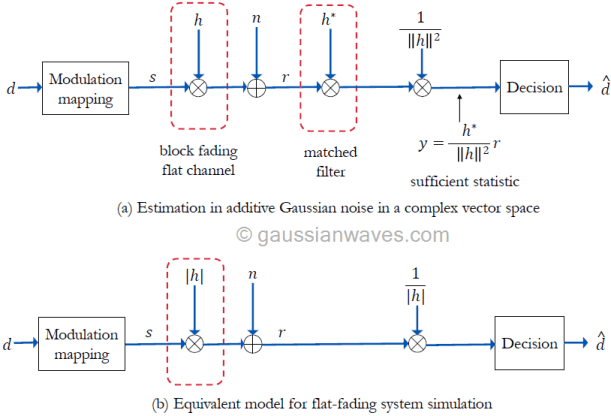
Simulation models for modulation and detection over a fading channel is shown in Figure 2. For a flat fading channel, the output of the channel can be expressed simply as the product of time varying channel response and the input signal. Thus, equation (1) can be simplified (refer this article for derivation) as follows for the flat fading channel.
Since the channel and noise are modeled as a complex vectors, the detection of \(\mathbf{s}\) from the received signal is an estimation problem in the complex vector space.
Assuming perfect channel knowledge at the receiver and coherent detection, the receiver shown in Figure 3(a) performs matched filtering. The impulse response of the matched filter is matched to the impulse response of the flat-fading channel as \( h^{\ast}\). The output of the matched filter is scaled down by a factor of \(||h||^2\) which is the total-energy contained in the impulse response of the flat-fading channel. The resulting decision vector \(\mathbf{y}\) serves as the sufficient statistic for the estimation of \(\mathbf{s}\) from the received signal \(\mathbf{r}\) (refer equation A.77 in reference [1])
Since the absolute value \(|h|\) and the Eucliden norm \(||h||\) are related as \(|h|^2= \left\lVert h\right\rVert = hh^{\ast}\), the model can be simplified further as given in Figure 3(b).
To simulate flat fading, the values for the fading variable \(h\) are drawn from complex normal distribution
\[h= X + jY \quad\quad (4) \]
where, \(X,Y\) are statistically independent real valued normal random variables.
● If \(E[h]=0\), then \(|h|\) is Rayleigh distributed, resulting in a Rayleigh flat fading channel ● If \(E[h] \neq 0\), then \(|h|\) is Rician distributed, resulting in a Rician flat fading channel with the factor \(K=[E[h]]^2/\sigma^2_h\)
The central limit theorem (CLT) is a fundamental concept in statistics and probability theory that explains how the sum of independent and identically distributed random variables behaves. The theorem states that as the number of these variables increases, the distribution of their sum tends to become more like a normal distribution, even if the variables themselves are not normally distributed.
CLT states that the sum of independent and identically distributed (i.i.d)random variables (with finite mean and variance) approaches normal distribution as sample size \(N \rightarrow \infty\). In simpler terms, the theorem states that under certain general conditions, the sum of independent observations that follow same underlying distribution approximates to normal distribution. The approximation steadily improves as the number of observations increase. The underlying distribution of the independent observation can be anything – binomial, Poisson, exponential, Chi-Squared etc.
Why CLT ?
CLT is an important concept in statistics because it allows us to make inferences about a population based on a sample, even if we do not know the distribution of the population. It is used in many statistical techniques, such as hypothesis testing and confidence intervals.
Applications of CLT
Central limit theorem (CLT) is applied in a vast range of applications including (but not limited to) signal processing, channel modeling, random process, population statistics, engineering research, predicting the confidence intervals, hypothesis testing, etc. One such application in signal processing is – deriving the response of a cascaded series of low pass filters by applying the CLT. In the article titled ‘the central limit theorem and low-pass filters‘ the author has illustrated how the response of a cascaded series of low pass filters approaches Gaussian shape as the number of filters in the series increase [1].
In digital communication, the effect of noise on a communication channel is modeled as additive Gaussian white noise. This follows from the fact that the noise from many physical channels can be considered approximately Gaussian. For example, the random movement of electrons in the semiconductor devices gives rise to shot noise whose effect can be approximated to Gaussian distribution by applying central limit theorem.
Law of large numbers and CLT
there is a connection between the central limit theorem and the law of large numbers.
The law of large numbers is another important theorem in probability theory, which states that as the number of independent and identically distributed (iid) random variables increases, the average of those variables converges to the expected value of the distribution. In other words, as the sample size increases, the sample mean becomes more and more representative of the true population mean.
The central limit theorem, on the other hand, describes the distribution of the sum of iid random variables, and shows that as the sample size increases, the distribution of the sum approaches a normal distribution.
Both the law of large numbers and the CLT deal with the behavior of the sum or average of iid random variables as the sample size gets larger. The law of large numbers describes the behavior of the sample mean, while the CLT describes the behavior of the sum of the variables.
In essence, the law of large numbers is a precursor to the central limit theorem, as it establishes the fact that the sample mean becomes more and more representative of the true population mean as the sample size increases, and the central limit theorem shows that the distribution of the sum of iid random variables approaches a normal distribution as the sample size gets larger.
The following Python code illustrate how the theorem comes to play when the number of observations is increased for two separate experiments: rolling \(N\) unbiased dice and tossing \(N\) unbiased coins. The code generates \(N\) i.i.d discrete uniform random variables that generates uniform random numbers from the set \(\left\{1,k\right\}\). In the case of the dice rolling experiment, \(k\) is set to \(6\), thus simulating the random pick from the sample space \(S=\left\{1,2,3,4,5,6\right\}\) with equal probability. For the coin tossing experiment, \(k\) is set to \(2\), thus simulating the sample space of \(S=\left\{1,2\right\}\) representing head or tail events with equal probability. Rest of the code is self explanatory.
Python code
#---------Central limit theorem - Author: Mathuranathan #gaussianwaves.com -----------------------
#
import numpy as np
import matplotlib.pyplot as plt
#%matplotlib inline

numIterations = np.asarray([1,2,5,10,50,100]); #number of i.i.d RVs
experiment = 'dice' #valid values: 'dice', 'coins'
maxNumForExperiment = {'dice':6,'coins':2} #max numbers represented on dice or coins
nSamp=100000

k = maxNumForExperiment[experiment]

fig, fig_axes = plt.subplots(ncols=3, nrows=2, constrained_layout=True)

for i,N in enumerate(numIterations):
    y = np.random.randint(low=1,high=k+1,size=(N,nSamp)).sum(axis=0)
    row = i//3;col=i%3;
    bins=np.arange(start=min(y),stop=max(y)+2,step=1)
    fig_axes[row,col].hist(y,bins=bins,density=True)
    fig_axes[row,col].set_title('N={} {}'.format(N,experiment))
plt.show()
Figure 1: Demonstrating central limit theorem using N numbers of dice
Figure 2: Demonstrating central limit theorem using N numbers of coins
Keywords: maximum likelihood decoding, digital communication, data storage, noise, interference, wireless communication systems, optical communication systems, digital storage systems, probability, likelihood estimation, python
Introduction
Maximum likelihood decoding is a technique used to determine the most likely transmitted message in a digital communicationsystem, based on the received signal and statistical models of noise and interference. The method uses maximum likelihood estimation to calculate the probability of each possible transmitted message and then selects the one with the highest probability.
To perform maximum likelihood decoding, the receiver uses a set of pre-defined models to estimate the likelihood of each possible transmitted message based on the received signal. The method is commonly used in various digital communication and data storage systems, such as wireless communication and digital storage. However, it can be complex and time-consuming, particularly in systems with large message spaces or complex noise and interference models.
Maximum Likelihood Decoding:
Consider a set of possible codewords (valid codewords – set \(Y\)) generated by an encoder in the transmitter side. We pick one codeword out of this set ( call it \(y\) ) and transmit it via a Binary Symmetric Channel (BSC) with probability of error \(p\) ( To know what is a BSC –click here). At the receiver side we receive the distorted version of \(y\) ( call this erroneous codeword \(x\)).
Maximum Likelihood Decoding chooses one codeword from \(Y\) (the list of all possible codewords) which maximizes the following probability.
\[\mathbb{P}(y\;sent\mid x\;received )\]
Meaning that the receiver computes \(P(y_1,x) , P(y_2,x) , P(y_3,x),\cdots,P(y_n,x)\). and chooses a codeword (\(y\)) which gives the maximum probability. In practice we don’t know \(y\) (at the receiver) but we know \(x\). So how to compute the probability ? Maximum Likelihood Estimation (MLE) comes to our rescue. For a detailed explanation on MLE – refer here[1] The aim of maximum likelihood estimation is to find the parameter value(s) that makes the observed data most likely. Understanding the difference between prediction and estimation is important at this point. Estimation differs from prediction in the following way … In estimation problems, likelihood of the parameters is estimated based on given data/observation vector. In prediction problems, probability is used as a measure to predict the outcome from known parameters of a model.
Examples for “Prediction” and “Estimation” :
1) Probability of getting a “Head” in a single toss of a fair coin is \(0.5\). The coin is tossed 100 times in a row.Prediction helps in predicting the outcome ( head or tail ) of the \(101^{th}\) toss based on the probability.
2) A coin is tossed 100 times and the data ( head or tail information) is recorded. Assuming the event follows Binomial distribution model, estimation helps in determining the probability of the event. The actual probability may or may not be \(0.5\). Maximum Likelihood Estimation estimates the conditional probability based on the observed data ( received data – \(x\)) and an assumed model.
Example of Maximum Likelihood Decoding:
Let \(y=11001001\) and \(x=10011001\) . Assuming Binomial distribution model for the event with probability of error \(0.1\) (i.e the reliability of the BSC is \(1-p = 0.9\)), the Hamming distance between codewords is \(2\) . For binomial model,
where \(d\) =the hamming distance between the received and the sent codewords n= number of bit sent \(p\)= error probability of the BSC. \(1-p\) = reliability of BSC
Substituting \(d=2, n=8\) and \(p=0.1\) , then \(P(y\;received \mid x\;sent) = 0.005314\).
Note : Here, Hamming distance is used to compute the probability. So the decoding can be called as “minimum distance decoding” (which minimizes the Hamming distance) or “maximum likelihood decoding”. Euclidean distance may also be used to compute the conditional probability.
As mentioned earlier, in practice \(y\) is not known at the receiver. Lets see how to estimate \(P(y \;received \mid x\; sent)\) when \(y\) is unknown based on the binomial model.
Since the receiver is unaware of the particular \(y\) corresponding to the \(x\) received, the receiver computes \(P(y\; received \mid x\; sent)\) for each codeword in \(Y\). The \(y\) which gives the maximum probability is concluded as the codeword that was sent.
Python code implementing Maximum Likelihood Decoding:
The following program for demonstrating the maximum likelihood decoding, involves generating a noisy signal from a transmitted message and then using maximum likelihood decoding to estimate the transmitted message from the noisy signal.
The maximum_likelihood_decoding function takes three arguments: received_signal, noise_variance, and message_space.
The calculate_probabilities function is called to calculate the probability of each possible message given the received signal, using the known noise variance.
The probabilities are normalized so that they sum to 1.
The maximum_likelihood_decoding function finds the index of the most likely message (i.e., the message with the highest probability).
The function returns the most likely message.
An example usage is demonstrated where a binary message space is defined ([0, 1]), along with a noise variance and a transmitted message.
The transmitted message is added to noise to generate a noisy received signal.
The maximum_likelihood_decoding function is called to decode the noisy signal.
The transmitted message, received signal, and decoded message are printed to the console for evaluation.
import numpy as np
import matplotlib.pyplot as plt

# Define a function to calculate the probability of each possible message given the received signal
def calculate_probabilities(received_signal, noise_variance, message_space):
    probabilities = np.zeros(len(message_space))

    for i, message in enumerate(message_space):
        error = received_signal - message
        probabilities[i] = np.exp(-np.sum(error ** 2) / (2 * noise_variance))

    return probabilities / np.sum(probabilities)

# Define a function to perform maximum likelihood decoding
def maximum_likelihood_decoding(received_signal, noise_variance, message_space):
    probabilities = calculate_probabilities(received_signal, noise_variance, message_space)
    most_likely_message_index = np.argmax(probabilities)
    return message_space[most_likely_message_index]

# Example usage
message_space = np.array([0, 1])
noise_variance = 0.4
transmitted_message = 1
received_signal = transmitted_message + np.sqrt(noise_variance) * np.random.randn()
decoded_message = maximum_likelihood_decoding(received_signal, noise_variance, message_space)

print('Transmitted message:', transmitted_message)
print('Received signal:', received_signal)
print('Decoded message:', decoded_message)

# Plot probability distribution
probabilities = calculate_probabilities(received_signal, noise_variance, message_space)
plt.bar(message_space, probabilities)
plt.title('Probability Distribution for Received Signal = {}'.format(received_signal))
plt.xlabel('Transmitted Message')
plt.ylabel('Probability')
plt.ylim([0, 1])
plt.show()
The probability of the received signal given a specific transmitted message is calculated as follows:
Compute the difference between the received signal and the transmitted message.
Compute the sum of squares of this difference vector.
Divide this sum by twice the known noise variance.
Take the negative exponential of this value.
This results in a probability density function (PDF) for the received signal given the transmitted message, assuming that the noise is Gaussian and zero-mean.
The probabilities for each possible transmitted message are then normalized so that they sum to 1. This is done by dividing each individual probability by the sum of all probabilities.
The maximum_likelihood_decoding function determines the most likely transmitted message by selecting the message with the highest probability, which corresponds to the maximum likelihood estimate of the transmitted message given the received signal and the statistical model of the noise.
Sample outputs
Transmitted message: 1
Received signal: 0.21798306949364643
Decoded message: 0

Transmitted message: 1
Received signal: -0.5115453787966966
Decoded message: 0

Transmitted message: 1
Received signal: 0.8343088336355061
Decoded message: 1

Transmitted message: 1
Received signal: -0.5479891887158619
Decoded message: 0
The probability distribution for the last sample output is shown below
Figure: Probability distribution for a sample run of the code
This website uses cookies to improve your experience while you navigate through the website. Out of these, the cookies that are categorized as necessary are stored on your browser as they are essential for the working of basic functionalities of the website. We also use third-party cookies that help us analyze and understand how you use this website. These cookies will be stored in your browser only with your consent. You also have the option to opt-out of these cookies. But opting out of some of these cookies may affect your browsing experience.
Necessary cookies are absolutely essential for the website to function properly. These cookies ensure basic functionalities and security features of the website, anonymously.
Cookie
Duration
Description
cookielawinfo-checbox-analytics
11 months
This cookie is set by GDPR Cookie Consent plugin. The cookie is used to store the user consent for the cookies in the category "Analytics".
cookielawinfo-checbox-analytics
11 months
This cookie is set by GDPR Cookie Consent plugin. The cookie is used to store the user consent for the cookies in the category "Analytics".
cookielawinfo-checbox-functional
11 months
The cookie is set by GDPR cookie consent to record the user consent for the cookies in the category "Functional".
cookielawinfo-checbox-functional
11 months
The cookie is set by GDPR cookie consent to record the user consent for the cookies in the category "Functional".
cookielawinfo-checbox-others
11 months
This cookie is set by GDPR Cookie Consent plugin. The cookie is used to store the user consent for the cookies in the category "Other.
cookielawinfo-checbox-others
11 months
This cookie is set by GDPR Cookie Consent plugin. The cookie is used to store the user consent for the cookies in the category "Other.
cookielawinfo-checkbox-necessary
11 months
This cookie is set by GDPR Cookie Consent plugin. The cookies is used to store the user consent for the cookies in the category "Necessary".
cookielawinfo-checkbox-performance
11 months
This cookie is set by GDPR Cookie Consent plugin. The cookie is used to store the user consent for the cookies in the category "Performance".
viewed_cookie_policy
11 months
The cookie is set by the GDPR Cookie Consent plugin and is used to store whether or not user has consented to the use of cookies. It does not store any personal data.
Functional cookies help to perform certain functionalities like sharing the content of the website on social media platforms, collect feedbacks, and other third-party features.
Performance cookies are used to understand and analyze the key performance indexes of the website which helps in delivering a better user experience for the visitors.
Analytical cookies are used to understand how visitors interact with the website. These cookies help provide information on metrics the number of visitors, bounce rate, traffic source, etc.


![x[n]](https://s0.wp.com/latex.php?latex=x%5Bn%5D&bg=ffffff&fg=000&s=0&c=20201002)

![X[z]](https://s0.wp.com/latex.php?latex=X%5Bz%5D&bg=ffffff&fg=000&s=0&c=20201002)